Machine Learning-Ex3(吴恩达课后习题)Multi-class Classification and Neural Networks

目录
1. Multi-class Classification
1.1 Dataset
1.2 Visualizing the data
1.3 Vectorizing Logistic Regression
1.3.1 Vectorizing the cost function(no regularization)
1.3.2 Vectorizing the gradient(no regularization)
1.3.3 Vectorizing regularized logistic regression
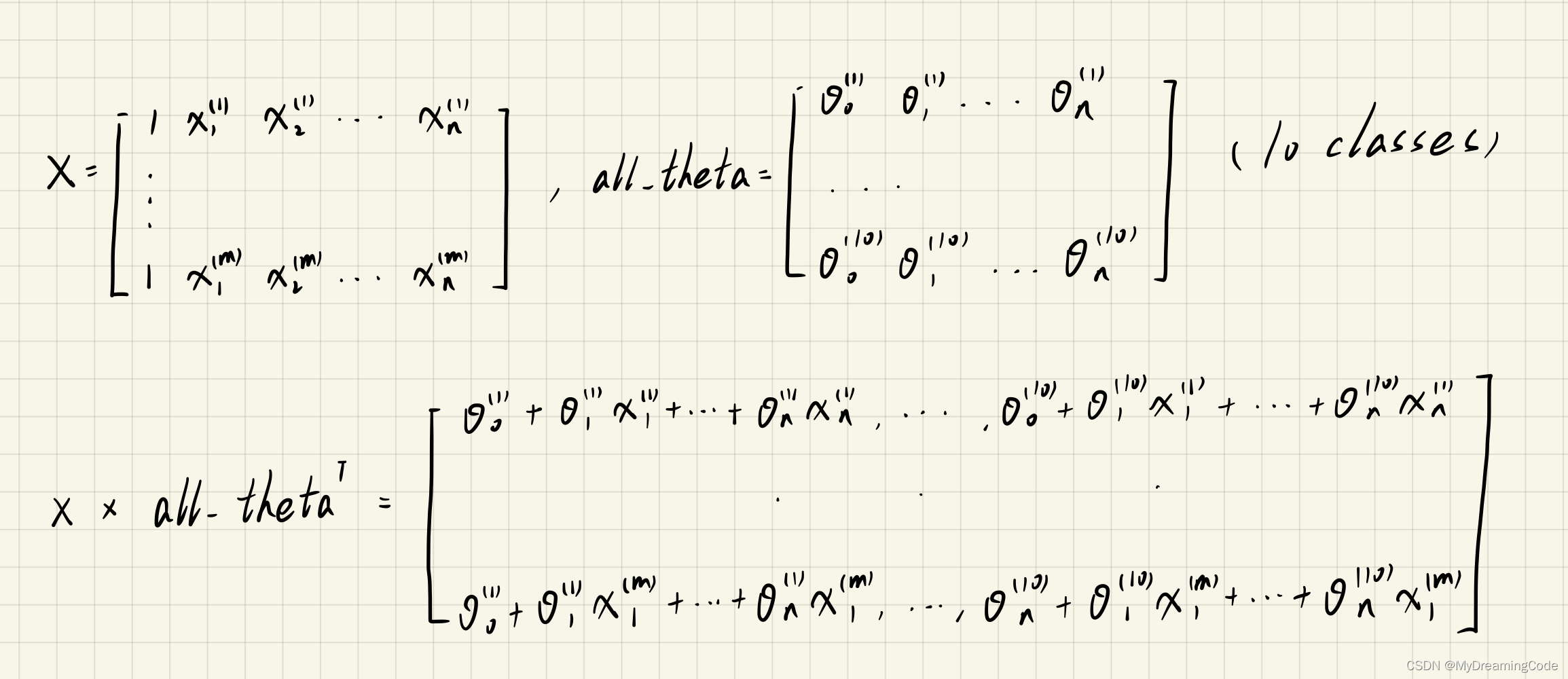
1.4 One-vs-all Classification
1.4.1 One-vs-all Prediction
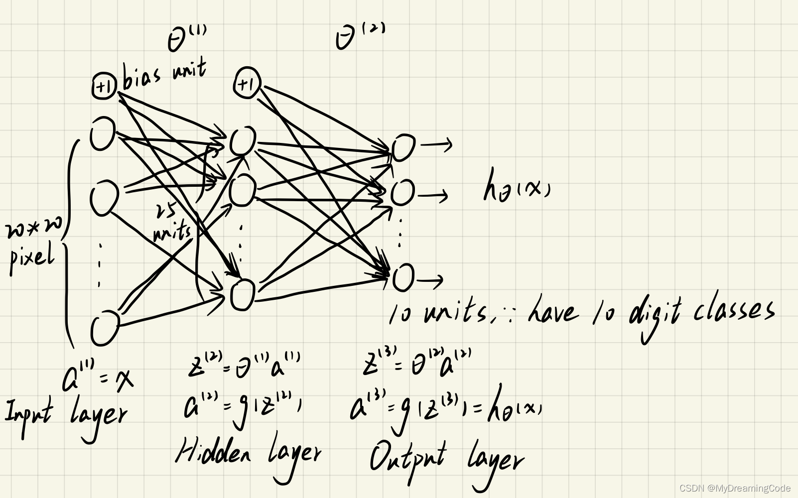
2. Neural Networks
2.1 Model representation
2.2 Feedforward Propagation and Prediction
1. Multi-class Classification
1.1 Dataset
内容:5000个20*20像素的手写字体图像与它对应的数字,其中数字0的值用10表示。
main.py
# scipy.io模块提供了很多函数来处理Matlab的数组
from scipy.io import loadmat  # loadmat方法可以导入Matlab格式数据data = loadmat('ex3data1.mat')
print(data)
print(data['X'].shape, data['y'].shape)  # (5000, 400) (5000, 1)
{'__header__': b'MATLAB 5.0 MAT-file, Platform: GLNXA64, Created on: Sun Oct 16 13:09:09 2011', '__version__': '1.0', '__globals__': [], 'X': array([[0., 0., 0., ..., 0., 0., 0.],
[0., 0., 0., ..., 0., 0., 0.],
[0., 0., 0., ..., 0., 0., 0.],
...,
[0., 0., 0., ..., 0., 0., 0.],
[0., 0., 0., ..., 0., 0., 0.],
[0., 0., 0., ..., 0., 0., 0.]]), 'y': array([[10],
[10],
[10],
...,
[ 9],
[ 9],
[ 9]], dtype=uint8)}
(5000, 400) (5000, 1)
1.2 Visualizing the data
内容:随机展示100个数据。
main.py
# scipy.io模块提供了很多函数来处理Matlab的数组
from scipy.io import loadmat  # loadmat方法可以导入Matlab格式数据
import numpy as npdata = loadmat('ex3data1.mat')
# np.random.choice(a,size=None,replace=True,p=None)
# 1.从a(必须是一维)中随机取数字,组成大小为size的数组;replace-True表示可以取相同数字;p-a中每个元素被取的概率,默认为每个元素概率相同
# np.arange(start,stop,step)用于生成数组-开始位置,停止位置,步长,即在给定间隔内返回均匀间隔的值
# print(np.arange(data['X'].shape[0]))  # [   0    1    2 ... 4997 4998 4999]
sample_index = np.random.choice(np.arange(data['X'].shape[0]), 100)  # 从0-4999中随机抽取100个数作为下标
sample_images = data['X'][sample_index, :]  # 抽取下标为sample_index的这些X的数据行
print(sample_images)
[[0. 0. 0. ... 0. 0. 0.]
[0. 0. 0. ... 0. 0. 0.]
[0. 0. 0. ... 0. 0. 0.]
...
[0. 0. 0. ... 0. 0. 0.]
[0. 0. 0. ... 0. 0. 0.]
[0. 0. 0. ... 0. 0. 0.]]
plot_training_set.py
import numpy as np
import matplotlib.pyplot as plt
import matplotlib  # 使用matplotlib.cm色表def plotTrainingSet(data):sample_index = np.random.choice(np.arange(data['X'].shape[0]), 100)  # 从0-4999中随机抽取100个数作为下标sample_images = data['X'][sample_index, :]  # 抽取下标为sample_index的这些X的数据行 (100*400)# subplots(nrows,ncols,sharex,sharey)-子图的行列数,sharex/sharey为True时所有子图共享x或y轴,为False时子图的x,y轴均为独立fig, axs = plt.subplots(nrows=10, ncols=10, sharex=True, sharey=True, figsize=(10, 10))# 1.使用axs[i][j]选中第i+1行j+1列的子图框# 2.matplotlib.pyplot.matshow(A,cmap),A-"矩阵"(一个矩阵元素对应一个图像像素),cmap-一种颜色映射方式# 3.matplotlib.cm为色表,binary为灰度图像标准色表,matshow为可绘制矩阵的函数# 4.xticks(ticks,labels),ticks-x轴刻度位置的列表,若传入空列表则不显示x轴,labels-放在指定刻度位置的标签文本for i in range(10):for j in range(10):axs[i][j].matshow(sample_images[i * 10 + j].reshape(20, 20).T, cmap=matplotlib.cm.binary)plt.xticks(np.array([]))plt.yticks(np.array([]))plt.show()
main.py
# scipy.io模块提供了很多函数来处理Matlab的数组
from scipy.io import loadmat  # loadmat方法可以导入Matlab格式数据
from plot_training_set import *  # 绘制训练集数据data = loadmat('ex3data1.mat')
plotTrainingSet(data)

1.3 Vectorizing Logistic Regression
内容:因为有10个数字类别,所以我们要做10个不同的逻辑回归分类器。将逻辑回归向量化会使训练效率更加高效。
1.3.1 Vectorizing the cost function(no regularization)
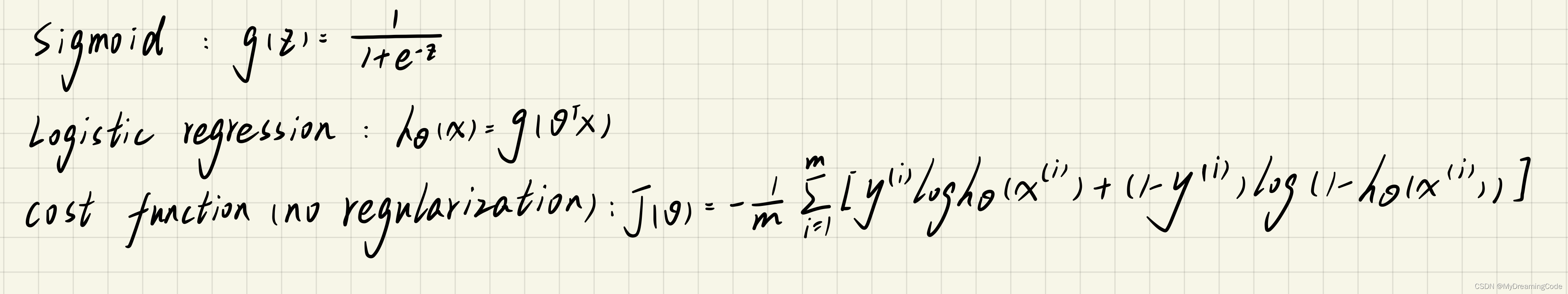
sigmoid.py
import numpy as np
def Sigmoid(z):return 1 / (1 + np.exp(-z))
cost_function.py(with regularization)
import numpy as np
from sigmoid import *def costFunction(theta, X, y, learningRate):theta = np.matrix(theta)X = np.matrix(X)y = np.matrix(y)m = len(X)first = np.multiply(y, np.log(Sigmoid(X * theta.T)))second = np.multiply(1 - y, np.log(1 - Sigmoid(X * theta.T)))reg = (learningRate / (2 * m)) * np.sum(np.power(theta[:, 1:theta.shape[1]], 2))  # theta0项不用正则化return np.sum(first + second) * (-1) / m + reg
1.3.2 Vectorizing the gradient(no regularization)
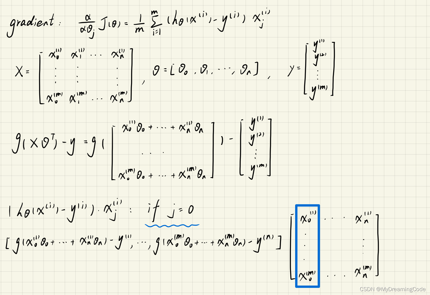
gradient.py
import numpy as np
from sigmoid import *def computeGradient(theta, X, y):X = np.matrix(X)y = np.matrix(y)theta = np.matrix(theta)m = len(X)grad = ((Sigmoid(X * theta.T) - y).T * X) / mreturn grad
1.3.3 Vectorizing regularized logistic regression

gradient.py
import numpy as np
from sigmoid import *def computeGradient(theta, X, y, learningRate):X = np.matrix(X)y = np.matrix(y)theta = np.matrix(theta)m = len(X)grad = ((((Sigmoid(X * theta.T) - y).T * X)).T + learningRate * theta.T) / mgrad[0][0] = (Sigmoid(X * theta.T) - y).T * X[:, 0] / mreturn grad
1.4 One-vs-all Classification
内容:构建分类器,由于逻辑回归只能在两个类别之间进行分类,所以我们需要多类分类的策略。对于每一个分类器我们只需要判断它的类别是'i'或者不是'i'即可。
one_vs_all.py
from scipy.optimize import minimize  # 提供最优化算法函数
import numpy as np
from cost_function import *  # 代价函数
from gradient import *  # 梯度def one_vs_all(X, y, num_labels, learningRate):rows = X.shape[0]cols = X.shape[1]all_theta = np.zeros((num_labels, cols + 1))  # 对于num_labels(10分类)的全部theta定义X = np.insert(X, 0, values=np.ones(rows), axis=1)  # 放入X0项,为1 (axis=1:按列放置)# 进行逻辑分类(做10个分类器)for i in range(1, num_labels + 1):theta = np.zeros(cols + 1)y_i = np.array([1 if label == i else 0 for label in y]).reshape(rows, 1)y_i = np.reshape(y_i, (rows, 1))# 1.fun:目标函数costFuntion# 2.x0:初始的猜测# 3.args=():优化的附加参数# 4.计算梯度的方法# method:要使用的方法名称,这里使用的TNC(截断牛顿算法)fmin = minimize(fun=costFunction, x0=theta, args=(X, y_i, learningRate), method='TNC', jac=computeGradient)all_theta[i - 1:] = fmin.x  # fmin.x是theta的值return all_theta
main.py
# scipy.io模块提供了很多函数来处理Matlab的数组
from scipy.io import loadmat  # loadmat方法可以导入Matlab格式数据
import numpy as np
from one_vs_all import *data = loadmat('ex3data1.mat')
X = data['X']
y = data['y']
theta = np.zeros(X.shape[1])
all_theta = one_vs_all(X, y, 10, 1)
print(all_theta)
[[-2.38358610e+00 0.00000000e+00 0.00000000e+00 ... 1.30435711e-03
-7.45365860e-10 0.00000000e+00]
[-3.18324551e+00 0.00000000e+00 0.00000000e+00 ... 4.45577193e-03
-5.07998907e-04 0.00000000e+00]
[-4.79716788e+00 0.00000000e+00 0.00000000e+00 ... -2.87443285e-05
-2.47862001e-07 0.00000000e+00]
...
[-7.98546406e+00 0.00000000e+00 0.00000000e+00 ... -8.95211947e-05
7.22094621e-06 0.00000000e+00]
[-4.57261766e+00 0.00000000e+00 0.00000000e+00 ... -1.33564925e-03
9.98868166e-05 0.00000000e+00]
[-5.40500039e+00 0.00000000e+00 0.00000000e+00 ... -1.16648642e-04
7.88651180e-06 0.00000000e+00]]
1.4.1 One-vs-all Prediction
内容:使用之前训练好的分类器来预测标签(概率最大的那一类即为标签,精确度可达94%)。
predict_all.py
import numpy as np
from sigmoid import *def predictAll(X, all_theta):rows = X.shape[0]X = np.insert(X, 0, values=np.ones(rows), axis=1)X = np.matrix(X)all_theta = np.matrix(all_theta)h_theta = Sigmoid(X * all_theta.T)# np.argmax(arr,axis)返回数组arr中最大值的索引值h_theta_max = np.argmax(h_theta, axis=1)return h_theta_max + 1
main.py
# scipy.io模块提供了很多函数来处理Matlab的数组
from scipy.io import loadmat  # loadmat方法可以导入Matlab格式数据
import numpy as np
from sklearn.metrics import classification_report  # 常用的输出模型评估报告方法
from one_vs_all import *
from predict_all import *  # 预测h_theta值data = loadmat('ex3data1.mat')
X = data['X']
y = data['y']
theta = np.zeros(X.shape[1])
all_theta = one_vs_all(X, y, 10, 1)
y_pred = predictAll(X, all_theta)
# classification_report(y_true,y_pred)y_true:真实值,y_pred:预测值
print(classification_report(y, np.array(y_pred)))
# precision recall f1-score support
# 精确率     召回率  调和平均数  支持度(指原始的真实数据中属于该类的个数)
precision recall f1-score support
1 0.95 0.99 0.97 500
2 0.95 0.92 0.93 500
3 0.95 0.91 0.93 500
4 0.95 0.95 0.95 500
5 0.92 0.92 0.92 500
6 0.97 0.98 0.97 500
7 0.95 0.95 0.95 500
8 0.93 0.92 0.92 500
9 0.92 0.92 0.92 500
10 0.97 0.99 0.98 500accuracy 0.94 5000
macro avg 0.94 0.94 0.94 5000
weighted avg 0.94 0.94 0.94 5000
2. Neural Networks
内容:神经网络可以处理比较复杂的非线性模型,这里给出了已经训练好的权重,我们使用前向传播即可。
2.1 Model representation
内容:
theta1:25*401 theta2:10*26
main.py
from scipy.io import loadmat
import numpy as npdata = loadmat('../ex3data1.mat')
X = np.matrix(data['X'])
X = np.insert(X, 0, values=np.ones(X.shape[0]), axis=1)  # axis=1即按列插入
y = np.matrix(data['y'])
weights = loadmat('ex3weights.mat')
theta1, theta2 = np.matrix(weights['Theta1']), np.matrix(weights['Theta2'])
print(theta1.shape, theta2.shape, X.shape, y.shape)
(25, 401) (10, 26) (5000, 401) (5000, 1)
2.2 Feedforward Propagation and Prediction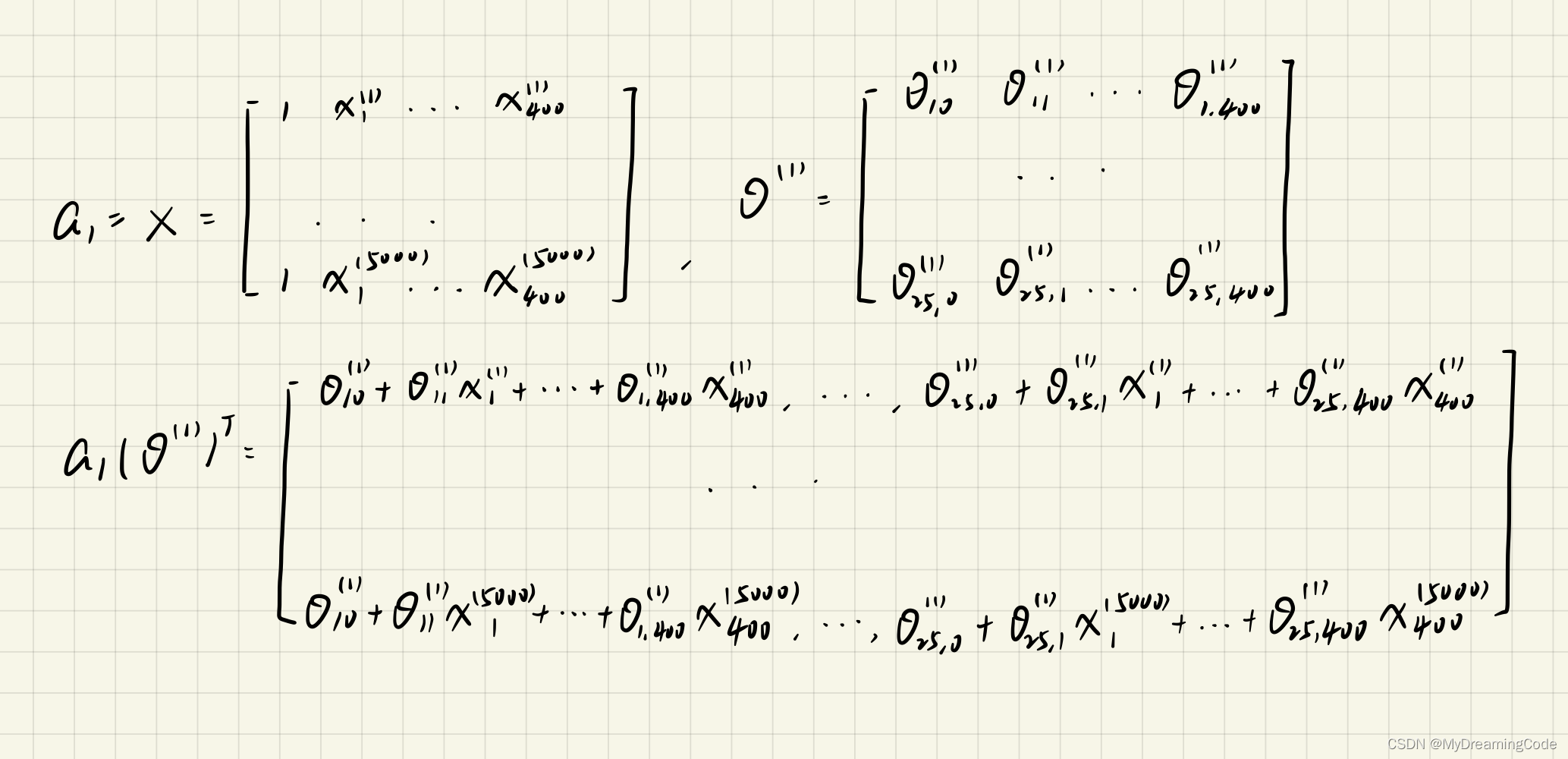
sigmoid.py
import numpy as npdef Sigmoid(z):return 1 / (1 + np.exp(-z))
main.py(输出a3,即h_theta的值)
from scipy.io import loadmat
import numpy as np
from sigmoid import *  # 激活函数data = loadmat('../ex3data1.mat')
X = np.matrix(data['X'])
X = np.insert(X, 0, values=np.ones(X.shape[0]), axis=1)  # axis=1即按列插入
y = np.matrix(data['y'])
weights = loadmat('ex3weights.mat')
theta1, theta2 = np.matrix(weights['Theta1']), np.matrix(weights['Theta2'])# 神经网络-前向反馈
a1 = X
z2 = a1 * theta1.T
# print(z2.shape)  # (5000, 25)
a2 = Sigmoid(z2)
a2 = np.insert(a2, 0, values=np.ones(a2.shape[0]), axis=1)  # 加偏置项,值为1
z3 = a2 * theta2.T
# print(z3.shape)  # (5000,10)
a3 = Sigmoid(z3)  # h_theta
print(a3)
[[1.12661530e-04 1.74127856e-03 2.52696959e-03 ... 4.01468105e-04
6.48072305e-03 9.95734012e-01]
[4.79026796e-04 2.41495958e-03 3.44755685e-03 ... 2.39107046e-03
1.97025086e-03 9.95696931e-01]
[8.85702310e-05 3.24266731e-03 2.55419797e-02 ... 6.22892325e-02
5.49803551e-03 9.28008397e-01]
...
[5.17641791e-02 3.81715020e-03 2.96297510e-02 ... 2.15667361e-03
6.49826950e-01 2.42384687e-05]
[8.30631310e-04 6.22003774e-04 3.14518512e-04 ... 1.19366192e-02
9.71410499e-01 2.06173648e-04]
[4.81465717e-05 4.58821829e-04 2.15146201e-05 ... 5.73434571e-03
6.96288990e-01 8.18576980e-02]]
进行预测(精确度可以达到97%):
main.py
from scipy.io import loadmat
from sklearn.metrics import classification_report
import numpy as np
from sigmoid import *  # 激活函数data = loadmat('../ex3data1.mat')
X = np.matrix(data['X'])
X = np.insert(X, 0, values=np.ones(X.shape[0]), axis=1)  # axis=1即按列插入
y = data['y']
weights = loadmat('ex3weights.mat')
theta1, theta2 = np.matrix(weights['Theta1']), np.matrix(weights['Theta2'])# 神经网络-前向反馈
a1 = X
z2 = a1 * theta1.T
a2 = Sigmoid(z2)
a2 = np.insert(a2, 0, values=np.ones(a2.shape[0]), axis=1)  # 加偏置项,值为1
z3 = a2 * theta2.T
a3 = Sigmoid(z3)  # h_theta
y_pred = np.argmax(a3, axis=1) + 1  # 每一项的预测值
print(classification_report(y, np.array(y_pred)))
precision recall f1-score support
1 0.97 0.98 0.98 500
2 0.98 0.97 0.98 500
3 0.98 0.96 0.97 500
4 0.97 0.97 0.97 500
5 0.97 0.98 0.98 500
6 0.98 0.99 0.98 500
7 0.98 0.97 0.97 500
8 0.98 0.98 0.98 500
9 0.97 0.96 0.96 500
10 0.98 0.99 0.99 500accuracy 0.98 5000
macro avg 0.98 0.98 0.98 5000
weighted avg 0.98 0.98 0.98 5000