前言

NeRF从2020年发展至今，仅仅三年时间，而Follow的工作已呈井喷之势，相信在不久的将来，NeRF会一举重塑三维重建这个业界，甚至重建我们的四维世界（开头先吹一波）。NeRF的发展时间虽短，有几篇工作却在研究领域开始呈现万精油趋势：

• PixelNeRF----泛化法宝
• MipNeRF----近远景重建
• NeRF in the wild----光线变换下的背景重建
• NeuS----用NeRF重建Surface
• Instant-NGP----多尺度Hash编码实现高效渲染

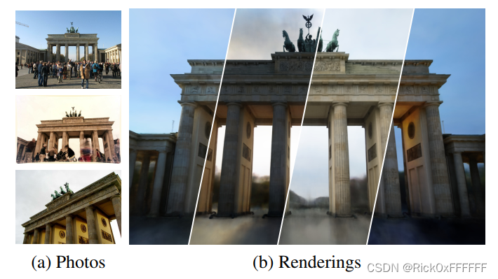
本篇是NeRF必读系列的最后一篇：NeRF in the Wild. 该篇主打一个Appearance Embedding, 由于该方法在生活场景中的普适性被大范围的使用，可以说再以后NeRF的文章中，NeRF-W将成为一篇难以避开的引用文章。

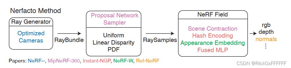
先插一句题外话，现在各行各业都流行一个通用的Framework, 例如搞detection的都有MMCV，MMDETECTION。基于Framework可以快速迭代自己的idea，在知识迅速爆炸的今天，学会各行各业的框架可谓是至关重要！所以在结束本期的paper解析之后，我将开启NeRFStudio系列的解析文章，开始NeRF领域的迅速迭代之旅！在此奉上NeRFStudio的pipeline，可以发现大部分文章我们都已经在前文中学习，仅剩下NeRF-W以及NeRF减减没有解析。下面补齐这两篇。

NeRF-W Main Contributions

1. Appearance Variations Embedding: 户外场景下被重建物体的曝光度，光线，季节、天气等的变换都会影响物体给出的appearance, 作者构造了一个Embedding层用来表征 ∇ V a p p r e a r a n c e \\nabla V_{apprearance} ∇Vapprearance​的低维描述
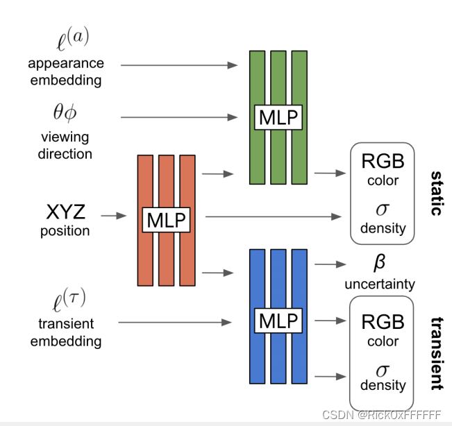
2. Transient Embedding：作者利用将一张图像分解为场景共享部分（shared elements）和依赖于图像的瞬息部分（transient elements，如名胜古迹照的游客）,并利用一个Transient Embedding层无监督地将这两个部分分解开来。具体的pipeline 如下：
   

经典Volumetric Rendering：

C ^ ( r ) = R ( r , c , σ ) = ∑ k = 1 K T ( t k ) α ( σ ( t k ) δ k ) c ( t k ) where  T ( t k ) = e x p ( − ∑ k ′ = 1 k − 1 σ ( t k ′ δ k ′ ) ) , \\hat{\\mathbf{C}}(\\mathbf{r})=\\mathcal{R}(\\mathbf{r, c},\\sigma)=\\sum^{K}_{k=1}T(t_k)\\alpha(\\sigma(t_k)\\delta_k)\\mathbf{c}(t_k)\\\\ \\text{where} \\space T(t_k)=exp(-\\sum^{k-1}_{k'=1}\\sigma(t_{k'}\\delta_{k'})), C^(r)=R(r,c,σ)=k=1∑K​T(tk​)α(σ(tk​)δk​)c(tk​)where T(tk​)=exp(−k′=1∑k−1​σ(tk′​δk′​)),
写成MLP的表达式如下：

[ σ ( t ) , z ( t ) ] = M L P θ 1 ( γ x ( r ( t ) ) ) c ( t ) = M L P θ 2 ( z t , γ d ( d ) ) \\begin{aligned} [\\sigma(t),\\bf{z}(t)]=MLP_{\\theta_1}(\\gamma_{\\bf{x}}(\\bf{r}(t))) \\\\ \\bf{c}(t)=MLP_{\\theta_2}(\\bf{z}_t,\\gamma_d(d)) \\end{aligned} [σ(t),z(t)]=MLPθ1​​(γx​(r(t)))c(t)=MLPθ2​​(zt​,γd​(d))​

作者为了强调$\sigma (t)$与观测角度无关，额外输出了隐变量$\mathbf{z}(t)$，做为根据$(\mathbf{x},\mathbf{d})$生成color的condition。
最后是Coarse And Fine Loss:
∑ i j ∥ C ( r i j ) − C ^ c ( r i j ) ∥ 2 2 + ∥ C ( r i j ) − C ^ f ( r i j ) ∥ 2 2 \\sum_{ij}\\Vert \\bf{C}(\\bf{r}_{ij}) -\\bf{\\hat{C}^c}(\\bf{r}_{ij}) \\Vert^2_{2}+\\Vert \\bf{C}(\\bf{r}_{ij}) -\\bf{\\hat{C}^f}(\\bf{r}_{ij}) \\Vert^2_{2} ij∑​∥C(rij​)−C^c(rij​)∥22​+∥C(rij​)−C^f(rij​)∥22​
以上便是经典的NeRF操作，下面作者开始介绍作者的魔改：

Latent Appearance Modeling

这一段在论文中4.1节，非常简约，作者给每张image分配了一个关联的隐编码 l i ( a ) \\mathcal{l}^{(a)}_i li(a)​, l i ( a ) \\mathcal{l}^{(a)}_i li(a)​会随着训练被优化，优化后的公式如下：
C ^ i ( r ) = R ( r , c , σ ) c i ( t ) = M L P θ 2 ( z t , γ d ( d ) , l i ( a ) ) \\hat{\\mathbf{C}}_i(\\mathbf{r})=\\mathcal{R}(\\mathbf{r, c},\\sigma)\\\\ \\bf{c}_i(t)=MLP_{\\theta_2}(\\bf{z}_t,\\gamma_d(d),\\mathcal{l}^{(a)}_i) C^i​(r)=R(r,c,σ)ci​(t)=MLPθ2​​(zt​,γd​(d),li(a)​)
关于 l i ( a ) \\mathcal{l}^{(a)}_i li(a)​的故事我会在后面详细述说，感兴趣的读者可以三连，点赞破10我加班更新，扑哧~

Transient Objects

瞬息物体对我们需要渲染的主体部分进行了遮挡，因此最后渲染图片的颜色也应该是不同的，作者按照这个思路增加了一个MLP， 并给出了改进后的渲染公式：
C ^ ( r ) = ∑ k = 1 K T ( t k ) ( α ( σ ( t k ) δ k ) c ( t k ) + α ( σ i ( τ ) ( t k ) δ k ) c i ( τ ) ( t k ) ) where  T i ( t k ) = e x p ( − ∑ k ′ = 1 k − 1 ( σ ( t k ′ ) + σ i ( τ ) ( t k ′ ) ) δ k ′ ) \\hat{\\mathbf{C}}(\\mathbf{r})=\\sum^{K}_{k=1}T(t_k)(\\alpha(\\sigma(t_k)\\delta_k)\\mathbf{c}(t_k)+\\alpha(\\sigma^{(\\tau)}_i(t_k)\\delta_k)\\mathbf{c}^{(\\tau)}_i(t_k))\\\\ \\text{where} \\space T_i(t_k)=exp(-\\sum^{k-1}_{k'=1}(\\sigma(t_{k'})+\\sigma^{(\\tau)}_i(t_{k'}))\\delta_{k'}) C^(r)=k=1∑K​T(tk​)(α(σ(tk​)δk​)c(tk​)+α(σi(τ)​(tk​)δk​)ci(τ)​(tk​))where Ti​(tk​)=exp(−k′=1∑k−1​(σ(tk′​)+σi(τ)​(tk′​))δk′​)
至此便能刻画出在存在Transient Objects的情况下，Volumetric Rendering的过程了，但作者并没有到此为止，更进一步的优化了Loss的分配比重。对于始终都是静态的图像区域，color的分布方差肯定较小，而transient objects较多的区域，color分布的方差会比较大，对于梯度的方向当然要多给跟方差变化较小的区域~
根据此思路，作者选择在渲染过程中直接估计方差 β ^ i ( r ) = R ( r , β i , σ i τ ) \\hat{\\beta}_i(\\mathbf{r})=\\mathcal{R}(\\mathbf{r},\\beta_i,\\sigma^{\\tau}_i) β^​i​(r)=R(r,βi​,σiτ​)

经过上述讨论，构建 MLP θ 3 \\text{MLP}_{\\theta_3} MLPθ3​​如下所示：
[ σ i ( τ ) ( t ) , c i ( τ ) ( t ) , β ~ i ( t ) ] = MLP θ 3 ( z ( t ) , l i ( τ ) ) β i ( t ) = β m i n + l o g ( 1 + e x p ( β ~ i ( t ) ) ) [\\sigma^{(\\tau)}_i(t),\\mathbf{c}^{(\\tau)}_i(t),\\tilde{\\beta}_i(t)]=\\text{MLP}_{\\theta_3}(\\mathbf{z}(t),\\mathcal{l}^{(\\tau)}_i)\\\\ \\beta_i(t)=\\beta_{min}+log(1+exp(\\tilde{\\beta}_i(t))) [σi(τ)​(t),ci(τ)​(t),β~​i​(t)]=MLPθ3​​(z(t),li(τ)​)βi​(t)=βmin​+log(1+exp(β~​i​(t)))
其中下式的意义是将输出从$(-\infty ,+\infty )$映射到$(0,+\infty )$，作者把上述loss构造给了fine model,而coarse model还是使用了经典loss
L i ( r ) = ∥ C i ( r ) − C ^ i ( r ) ∥ 2 2 2 β i ( r ) 2 + l o g β i ( r ) 2 2 + λ μ K ∑ k = 1 K σ i ( τ ) ( t k ) L t o t a l = ∑ i j L i ( r i j ) + 1 2 ∥ C ( r i j ) − C ^ i c ( r i j ) ∥ L_i(\\bm{r})=\\frac{\\Vert\\bm{C}_i(\\bm{r})-\\hat{\\bm{C}}_i(\\bm{r})\\Vert^2_2}{2\\beta_i(\\bm{r})^2}+\\frac{log\\beta_i(\\bm{r})^2}{2}+\\frac{\\lambda_\\mu}{K}\\sum^K_{k=1}\\sigma^{(\\tau)}_i(t_k)\\\\ L_{total}=\\sum_{ij}L_i(\\bm{r}_{ij})+\\frac{1}{2}\\Vert C(\\bm{r}_{ij})-\\hat{C}^c_i(\\bm{r}_{ij})\\Vert Li​(r)=2βi​(r)2∥Ci​(r)−C^i​(r)∥22​​+2logβi​(r)2​+Kλμ​​k=1∑K​σi(τ)​(tk​)Ltotal​=ij∑​Li​(rij​)+21​∥C(rij​)−C^ic​(rij​)∥

参考文献

Martin-Brualla, Ricardo, et al. “Nerf in the wild: Neural radiance fields for unconstrained photo collections.” Proceedings of the IEEE/CVF Conference on Computer Vision and Pattern Recognition. 2021.