DeepSORT中的卡尔曼滤波

本文是看了DeepSORT方法视频之后,关于其中使用的卡尔曼滤波的理解
DeepSORT视频链接
首先是视频中的一张图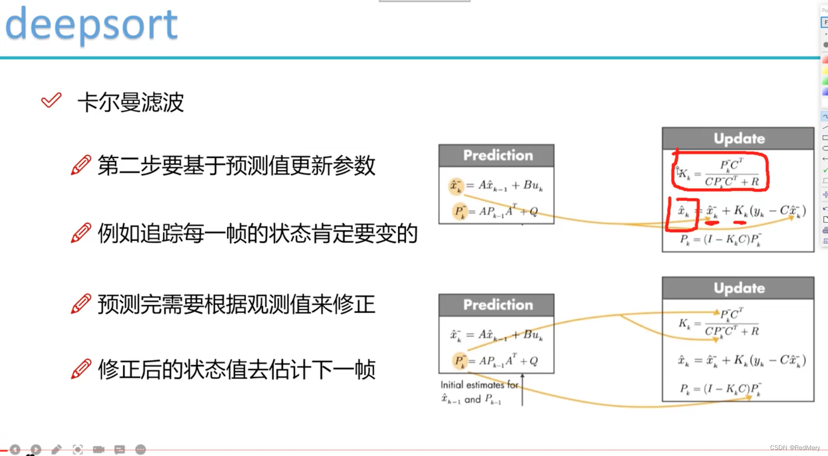
预测阶段
x ^ k − = A x ^ k − 1 \\hat{x}_k^-=A\\hat{x}_{k-1} x^k−=Ax^k−1
P k − = A P k − 1 + Q , P k − ∈ R 8 , 8 P_k^-=AP_{k-1}+Q, P_k^- \\in R^{8,8} Pk−=APk−1+Q,Pk−∈R8,8
更新阶段
K k = P k − C T C P k − C T + R , K k ∈ R 8 , 4 K_k=\\frac{P_k^-C^T}{CP_k^-C^T+R}, K_k\\in R^{8,4} Kk=CPk−CT+RPk−CT,Kk∈R8,4
x k ^ = x ^ k − + K k ( y k − C x ^ k − ) , C ∈ R 4 , 8 , x ^ k − ∈ R 8 , 1 , y k ∈ R 4 , 1 \\hat{x_k}=\\hat{x}_k^-+K_k(y_k-C\\hat{x}_k^-), C\\in R^{4,8}, \\hat{x}_k^-\\in R^{8,1}, y_k\\in R^{4,1} xk^=x^k−+Kk(yk−Cx^k−),C∈R4,8,x^k−∈R8,1,yk∈R4,1
P k = ( I − K k C ) P k − P_k=(I-K_kC)P_k^- Pk=(I−KkC)Pk−
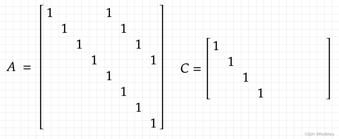
整个过程中,矩阵A和矩阵C保持不变,具体如下所示。C是状态观测矩阵,比如,如果我们现在的观测值是速度,而需要的是位置,那么C就是由速度变化到位置的变换矩阵。而在这里,C是由检测框变换到检测框的变换矩阵,因此C里都是1
 详细步骤:
详细步骤:
1.获得第一帧输出的检测框参数初始化
x ^ k − \\hat{x}_k^- x^k−和 P k − P_k^- Pk−首先被初始化
x ^ 0 − = [ x , y , r , h , 0 , 0 , 0 , 0 ] , ∈ R 1 , 8 \\hat{x}_0^-=[x,y,r,h,0,0,0,0], \\in R^{1,8} x^0−=[x,y,r,h,0,0,0,0],∈R1,8
P k − P_k^- Pk−与 x ^ 0 − , ∈ R 8 , 8 \\hat{x}_0^-, \\in R^{8,8} x^0−,∈R8,8 有关,差了一个系数,代码如下所示
# self._std_weight_position = 0.05
# self._std_weight_velocity = 0.00625
std = [2 * self._std_weight_position * measurement[3],   #2 * self._std_weight_position * measurement[3],    1e-2,    2 * self._std_weight_position * measurement[3],     10 * self._std_weight_velocity * measurement[3],    10 * self._std_weight_velocity * measurement[3],   1e-5,    10 * self._std_weight_velocity * measurement[3]]
covariance = np.diag(np.square(std))
2.预测下一时刻(第二帧中检测框的位置,图中的Prediction过程)
x ^ k − \\hat{x}_k^- x^k−正常计算,
P k − 中的 Q P_k^-中的 Q Pk−中的Q是一个随机噪声,其为
std_pos = [ self._std_weight_position * mean[3], self._std_weight_position * mean[3], 1e-2, self._std_weight_position * mean[3]] std_vel = [self._std_weight_velocity * mean[3], self._std_weight_velocity * mean[3], 1e-5, self._std_weight_velocity * mean[3]] motion_cov = np.diag(np.square(np.r_[std_pos, std_vel])) mean = np.dot(self._motion_mat, mean)covariance = np.linalg.multi_dot(( self._motion_mat, covariance, self._motion_mat.T)) + motion_cov
3.完成配对,给每一个轨迹匹配一个检测框
4.更新过程(Update)
def project(self, mean, covariance): """Project state distribution to measurement space. Parameters ---------- mean : ndarray The state's mean vector (8 dimensional array). covariance : ndarray The state's covariance matrix (8x8 dimensional). Returns ------- (ndarray, ndarray) Returns the projected mean and covariance matrix of the given state estimate. """ std = [ self._std_weight_position * mean[3], self._std_weight_position * mean[3], 1e-1, self._std_weight_position * mean[3]] innovation_cov = np.diag(np.square(std)) mean = np.dot(self._update_mat, mean) covariance = np.linalg.multi_dot(( self._update_mat, covariance, self._update_mat.T)) return mean, covariance + innovation_covdef update(self, mean, covariance, measurement): """Run Kalman filter correction step. Parameters ---------- mean : ndarray The predicted state's mean vector (8 dimensional). covariance : ndarray The state's covariance matrix (8x8 dimensional). measurement : ndarray The 4 dimensional measurement vector (x, y, a, h), where (x, y) is the center position, a the aspect ratio, and h the height of the bounding box. Returns ------- (ndarray, ndarray) Returns the measurement-corrected state distribution. """ projected_mean, projected_cov = self.project(mean, covariance) #求解AX=b中的xchol_factor, lower = scipy.linalg.cho_factor(projected_cov, lower=True, check_finite=False) kalman_gain = scipy.linalg.cho_solve((chol_factor,lower), np.dot(covariance, self._update_mat.T).T, check_finite=False).T innovation = measurement - projected_mean new_mean = mean + np.dot(innovation, kalman_gain.T) new_covariance = covariance - np.linalg.multi_dot(( kalman_gain, projected_cov, kalman_gain.T)) return new_mean, new_covariance
然后不断的完成上述步骤