【数据挖掘与商务智能决策】第十一章 AdaBoost与GBDT模型

11.1 AdaBoost模型简单代码实现
1.AdaBoost分类模型演示
from sklearn.ensemble import AdaBoostClassifier
X = [[1, 2], [3, 4], [5, 6], [7, 8], [9, 10]]
y = [0, 0, 0, 1, 1]model = AdaBoostClassifier(random_state=123)
model.fit(X, y)print(model.predict([[5, 5]]))
[0]
2.AdaBoost回归模型演示
from sklearn.ensemble import AdaBoostRegressor
X = [[1, 2], [3, 4], [5, 6], [7, 8], [9, 10]]
y = [1, 2, 3, 4, 5]model = AdaBoostRegressor(random_state=123)
model.fit(X, y)print(model.predict([[5, 5]]))
[3.]
11.2 案例实战 - AdaBoost信用卡精准营销模型
11.2.2 模型搭建
1.读取数据
import pandas as pd
df = pd.read_excel('信用卡精准营销模型.xlsx')
df.head()
| 年龄 | 月收入(元) | 月消费(元) | 性别 | 月消费/月收入 | 响应 | |
|---|---|---|---|---|---|---|
| 0 | 30 | 7275 | 6062 | 0 | 0.833265 | 1 |
| 1 | 25 | 17739 | 13648 | 0 | 0.769378 | 1 |
| 2 | 29 | 25736 | 14311 | 0 | 0.556069 | 1 |
| 3 | 23 | 14162 | 7596 | 0 | 0.536365 | 1 |
| 4 | 27 | 15563 | 12849 | 0 | 0.825612 | 1 |
2.提取特征变量和目标变量
X = df.drop(columns='响应')
y = df['响应']
3.划分训练集和测试集
from sklearn.model_selection import train_test_split
X_train, X_test, y_train, y_test = train_test_split(X, y, test_size=0.2, random_state=123)
4.模型训练及搭建
from sklearn.ensemble import AdaBoostClassifier
clf = AdaBoostClassifier(random_state=123)
clf.fit(X_train, y_train)
AdaBoostClassifier(random_state=123)
In a Jupyter environment, please rerun this cell to show the HTML representation or trust the notebook.
On GitHub, the HTML representation is unable to render, please try loading this page with nbviewer.org.
AdaBoostClassifier(random_state=123)
11.2.3 模型预测及评估
# 模型搭建完毕后,通过如下代码预测测试集数据:
y_pred = clf.predict(X_test)
print(y_pred)
[1 1 1 0 1 0 1 0 0 0 1 1 1 1 1 0 0 1 1 0 1 1 1 1 0 0 0 0 0 0 0 0 0 1 0 1 01 1 0 0 0 1 1 0 0 1 0 0 0 1 0 0 0 1 1 0 0 0 1 0 0 0 0 0 0 0 0 0 1 1 0 0 10 0 0 0 1 0 0 1 0 1 0 1 0 1 0 0 0 0 0 0 0 1 0 0 0 0 0 0 0 0 0 0 1 0 0 1 10 1 0 1 0 0 0 1 0 0 0 1 0 0 1 0 1 1 1 0 0 0 0 0 0 0 1 0 0 0 0 1 1 1 0 0 10 1 0 1 0 0 0 0 0 1 1 0 1 0 1 1 1 0 0 1 1 0 0 0 0 1 0 1 0 0 0 1 0 1 0 1 10 0 1 0 0 0 0 0 0 0 1 1 0 1 1]
# 通过和之前章节类似的代码,我们可以将预测值和实际值进行对比:
a = pd.DataFrame()  # 创建一个空DataFrame
a['预测值'] = list(y_pred)
a['实际值'] = list(y_test)
a.head()
| 预测值 | 实际值 | |
|---|---|---|
| 0 | 1 | 1 |
| 1 | 1 | 1 |
| 2 | 1 | 1 |
| 3 | 0 | 0 |
| 4 | 1 | 1 |
# 查看预测准确度
from sklearn.metrics import accuracy_score
score = accuracy_score(y_pred, y_test)
print(score)
0.85
#查看预测分类概率
y_pred_proba = clf.predict_proba(X_test)
y_pred_proba[0:5]  # 查看前5项,第一列为分类为0的概率,第二列为分类为1的概率
array([[0.19294615, 0.80705385],[0.41359387, 0.58640613],[0.42597039, 0.57402961],[0.66817389, 0.33182611],[0.32850159, 0.67149841]])
%matplotlib inline
# 绘制ROC曲线
from sklearn.metrics import roc_curve
fpr, tpr, thres = roc_curve(y_test.values, y_pred_proba[:,1])
import matplotlib.pyplot as plt
plt.plot(fpr, tpr)
plt.show()
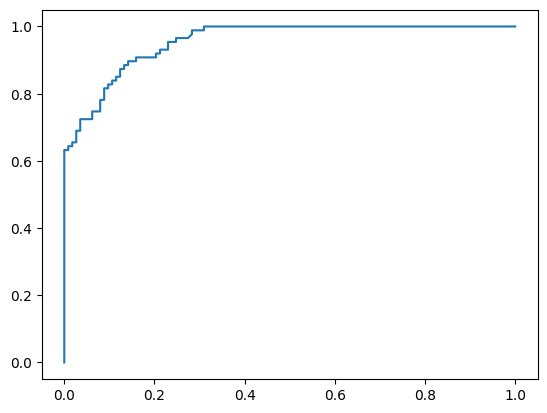
# 查看AUC值
from sklearn.metrics import roc_auc_score
score = roc_auc_score(y_test, y_pred_proba[:,1])
print(score)
0.9559047909673483
# 查看特征重要性
clf.feature_importances_
array([0.18, 0.2 , 0.36, 0.02, 0.24])
# 通过DataFrame的方式展示特征重要性
features = X.columns  # 获取特征名称
importances = clf.feature_importances_  # 获取特征重要性# 通过二维表格形式显示
importances_df = pd.DataFrame()
importances_df['特征名称'] = features
importances_df['特征重要性'] = importances
importances_df.sort_values('特征重要性', ascending=False)
| 特征名称 | 特征重要性 | |
|---|---|---|
| 2 | 月消费(元) | 0.36 |
| 4 | 月消费/月收入 | 0.24 |
| 1 | 月收入(元) | 0.20 |
| 0 | 年龄 | 0.18 |
| 3 | 性别 | 0.02 |
11.2.4 模型参数(选学)
# # 分类模型,通过如下代码可以查看官方介绍
# from sklearn.ensemble import AdaBoostClassifier
# AdaBoostClassifier?
# # 回归模型,通过如下代码可以查看官方介绍
# from sklearn.ensemble import AdaBoostRegressor
# AdaBoostRegressor?
11.3 GBDT算法的简单代码实现
1.GBDT分类模型演示
from sklearn.ensemble import GradientBoostingClassifier
X = [[1, 2], [3, 4], [5, 6], [7, 8], [9, 10]]
y = [0, 0, 0, 1, 1]model = GradientBoostingClassifier(random_state=123)
model.fit(X, y)print(model.predict([[5, 5]]))
[0]
2.GBDT回归模型演示
from sklearn.ensemble import GradientBoostingRegressor
X = [[1, 2], [3, 4], [5, 6], [7, 8], [9, 10]]
y = [1, 2, 3, 4, 5]model = GradientBoostingRegressor(random_state=123)
model.fit(X, y)print(model.predict([[5, 5]]))
[2.54908866]
11.4 GBDT案例实战 - 产品定价模型
11.4.2 模型搭建
1.读取数据
import pandas as pd
df = pd.read_excel('产品定价模型.xlsx')
df.head()
| 页数 | 类别 | 彩印 | 纸张 | 价格 | |
|---|---|---|---|---|---|
| 0 | 207 | 技术类 | 0 | 双胶纸 | 60 |
| 1 | 210 | 技术类 | 0 | 双胶纸 | 62 |
| 2 | 206 | 技术类 | 0 | 双胶纸 | 62 |
| 3 | 218 | 技术类 | 0 | 双胶纸 | 64 |
| 4 | 209 | 技术类 | 0 | 双胶纸 | 60 |
查看各个分类的数据量
df['类别'].value_counts()
技术类    336
教辅类    333
办公类    331
Name: 类别, dtype: int64
df['彩印'].value_counts()
0    648
1    352
Name: 彩印, dtype: int64
df['纸张'].value_counts()
双胶纸    615
铜版纸    196
书写纸    189
Name: 纸张, dtype: int64
2.分类型文本变量处理
将文本内容转为数值,关于LabelEncoder()函数也在将在11.1.2节进行进一步讲解
from sklearn.preprocessing import LabelEncoder
le = LabelEncoder()
df['类别'] = le.fit_transform(df['类别'])  # 处理类别
# 将类别一列处理后,我们可以使用value_counts()方法查看转化效果:
df['类别'].value_counts()
1    336
2    333
0    331
Name: 类别, dtype: int64
# 另外一种文本内容转为数值的方法,注意不要再运行完上面的代码后运行,因为上面的内容已经被替代完毕了,如果想尝试,需要重新运行,并且,先运行下面的代码
# df['类别'] = df['类别'].replace({'办公类': 0, '技术类': 1, '教辅类': 2})
# df['类别'].value_counts()
# 下面我们使用同样的方法处理“纸张”一列:
le = LabelEncoder()
df['纸张'] = le.fit_transform(df['纸张'])
# 此时的表格如下:
df.head()
| 页数 | 类别 | 彩印 | 纸张 | 价格 | |
|---|---|---|---|---|---|
| 0 | 207 | 1 | 0 | 1 | 60 |
| 1 | 210 | 1 | 0 | 1 | 62 |
| 2 | 206 | 1 | 0 | 1 | 62 |
| 3 | 218 | 1 | 0 | 1 | 64 |
| 4 | 209 | 1 | 0 | 1 | 60 |
3.提取特征变量和目标变量
X = df.drop(columns='价格')
y = df['价格']
4.划分训练集和测试集
from sklearn.model_selection import train_test_split
X_train, X_test, y_train, y_test = train_test_split(X, y, test_size=0.2, random_state=123)
5.模型训练及搭建
from sklearn.ensemble import GradientBoostingRegressor
model = GradientBoostingRegressor(random_state=123)
model.fit(X_train, y_train)
GradientBoostingRegressor(random_state=123)
In a Jupyter environment, please rerun this cell to show the HTML representation or trust the notebook.
On GitHub, the HTML representation is unable to render, please try loading this page with nbviewer.org.
GradientBoostingRegressor(random_state=123)
11.4.3 模型预测及评估
# 模型搭建完毕后,通过如下代码预测测试集数据:
y_pred = model.predict(X_test)
print(y_pred[0:50])
[ 71.15004038 79.56199921 68.21751792 90.78788507 78.8847912842.28022702 39.27334177 60.74670841 53.59744659 77.6593177180.22295545 76.04437155 79.56199921 58.40372895 79.6524526644.27997693 53.18177447 35.31452467 92.1798291 58.4037289541.96644278 99.50466356 80.22295545 79.69648341 91.4506174142.93885741 42.86973046 75.71824996 48.55203652 62.9418577839.47077874 61.54190648 95.18389309 51.88118394 65.129313950.17577837 39.54495179 83.63542315 56.24632221 102.117611248.89080247 49.23639342 33.03502962 52.74862135 35.4722086735.00370671 53.9446399 74.62364353 35.31452467 53.9446399 ]
# 通过和之前章节类似的代码,我们可以将预测值和实际值进行对比:
a = pd.DataFrame()  # 创建一个空DataFrame
a['预测值'] = list(y_pred)
a['实际值'] = list(y_test)
a.head()
| 预测值 | 实际值 | |
|---|---|---|
| 0 | 71.150040 | 75 |
| 1 | 79.561999 | 84 |
| 2 | 68.217518 | 68 |
| 3 | 90.787885 | 90 |
| 4 | 78.884791 | 85 |
# 查看预测评分 - 方法1:自带的score函数,本质就是R-squared值(也即统计学中常说的R^2)
model.score(X_test, y_test)
0.8741691363311168
# 查看预测评分 - 方法2:r2_score()函数
from sklearn.metrics import r2_score
r2 = r2_score(y_test, model.predict(X_test))
print(r2)
0.8741691363311168
# 查看特征重要性
model.feature_importances_
array([0.49070203, 0.44718694, 0.04161545, 0.02049558])
# 通过DataFrame的方式展示特征重要性
features = X.columns  # 获取特征名称
importances = model.feature_importances_  # 获取特征重要性# 通过二维表格形式显示
importances_df = pd.DataFrame()
importances_df['特征名称'] = features
importances_df['特征重要性'] = importances
importances_df.sort_values('特征重要性', ascending=False)
| 特征名称 | 特征重要性 | |
|---|---|---|
| 0 | 页数 | 0.490702 |
| 1 | 类别 | 0.447187 |
| 2 | 彩印 | 0.041615 |
| 3 | 纸张 | 0.020496 |
11.4.4 模型参数(选学)
# # 分类模型,通过如下代码可以查看官方介绍
# from sklearn.ensemble import AdaBoostClassifier
# AdaBoostClassifier?
# # 回归模型,通过如下代码可以查看官方介绍
# from sklearn.ensemble import AdaBoostRegressor
# AdaBoostRegressor?