「解析」Matplotlib 绘制折线图

相比于【优雅】matplotlib 常见图、【优雅】matplotlib 3D图 而言,折线图使用的频率会更高一些,在此整理下最近使用 Matplotlib 绘制折线图常用的一些配置,小伙伴们只需要修改对应的 aug_list、list 即可直接使用
# !/usr/bin/env python
# -*- coding:utf-8 -*-
# @Time : 2023.04
# @Author : 绿色羽毛
# @Email : lvseyumao@foxmail.com
# @Blog : https://blog.csdn.net/ViatorSun
# @arXiv :
# @version : "1.0"
# @Note :
#
#import numpy as np
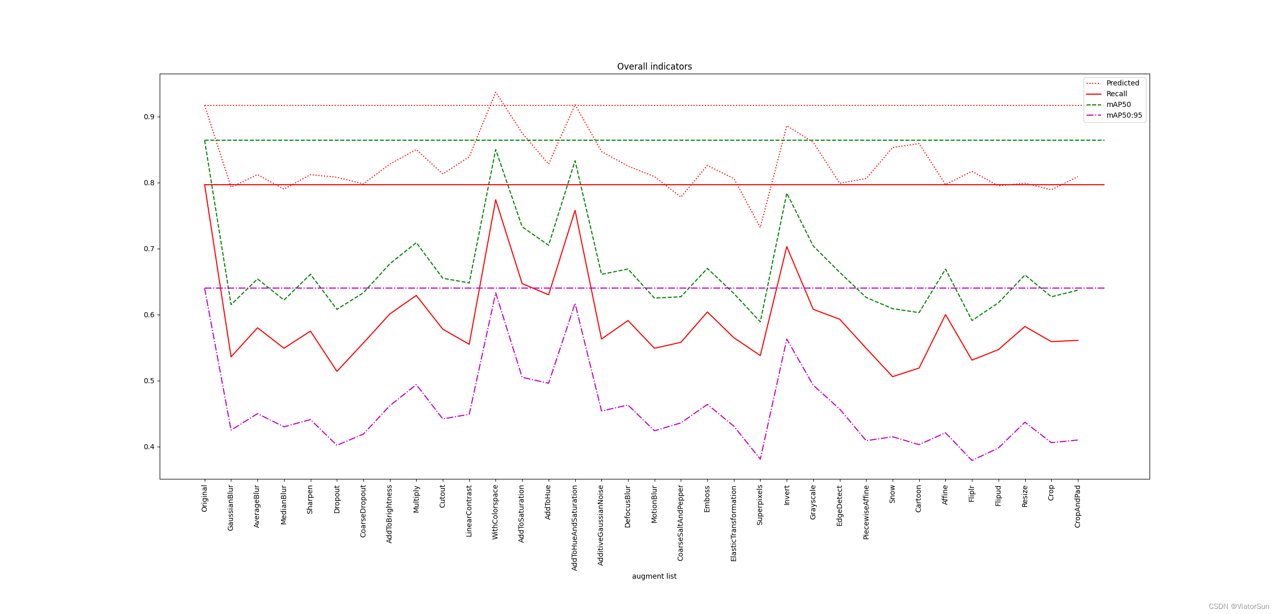
import matplotlib.pyplot as pltaug_list=[ "Original","GaussianBlur", "AverageBlur", "MedianBlur", "Sharpen", "Dropout","CoarseDropout", "AddToBrightness", "Multiply", "Cutout", "LinearContrast", "WithColorspace", "AddToSaturation","AddToHue", "AddToHueAndSaturation", "AdditiveGaussianNoise", "DefocusBlur",# GPU 1"MotionBlur", "CoarseSaltAndPepper","Emboss", "ElasticTransformation", "Superpixels", "Invert", "Grayscale", "EdgeDetect", "PiecewiseAffine", "Snow", "Cartoon", "Affine", "Fliplr", "Flipud", "Resize", "Crop", "CropAndPad", ]list = ["| 0 | Original | 0.917 | 0.797 | 0.864 | 0.64 |","| 1 | GaussianBlur | 0.793 | 0.536 | 0.615 | 0.425 |","| 2 | AverageBlur | 0.812 | 0.58 | 0.654 | 0.45 |","| 3 | MedianBlur | 0.79 | 0.549 | 0.622 | 0.43 |","| 4 | Sharpen | 0.812 | 0.575 | 0.661 | 0.441 |","| 5 | Dropout | 0.808 | 0.514 | 0.608 | 0.402 |","| 6 | CoarseDropout | 0.798 | 0.557 | 0.633 | 0.419 |","| 7 | AddToBrightness | 0.828 | 0.601 | 0.677 | 0.462 |","| 8 | Multiply | 0.85 | 0.629 | 0.709 | 0.494 |","| 9 | Cutout | 0.813 | 0.578 | 0.655 | 0.442 |","| 10 | LinearContrast | 0.839 | 0.555 | 0.648 | 0.449 |","| 11 | WithColorspace | 0.937 | 0.774 | 0.85 | 0.633 |","| 12 | AddToSaturation | 0.875 | 0.647 | 0.733 | 0.505 |","| 13 | AddToHue | 0.828 | 0.63 | 0.705 | 0.496 |","| 14 | AddToHueAndSaturation | 0.918 | 0.758 | 0.833 | 0.617 |","| 15 | AdditiveGaussianNoise | 0.847 | 0.563 | 0.661 | 0.454 |","| 16 | DefocusBlur | 0.825 | 0.591 | 0.669 | 0.463 |","| 17 | MotionBlur | 0.809 | 0.549 | 0.625 | 0.424 |","| 18 | CoarseSaltAndPepper | 0.778 | 0.558 | 0.627 | 0.436 |","| 19 | Emboss | 0.826 | 0.604 | 0.67 | 0.464 |","| 20 | ElasticTransformation | 0.806 | 0.565 | 0.632 | 0.431 |","| 21 | Superpixels | 0.732 | 0.538 | 0.589 | 0.381 |","| 22 | Invert | 0.886 | 0.703 | 0.784 | 0.563 |","| 23 | Grayscale | 0.861 | 0.608 | 0.704 | 0.493 |","| 24 | EdgeDetect | 0.799 | 0.593 | 0.664 | 0.457 |","| 25 | PiecewiseAffine | 0.806 | 0.549 | 0.626 | 0.409 |","| 26 | Snow | 0.853 | 0.506 | 0.609 | 0.415 |","| 27 | Cartoon | 0.859 | 0.519 | 0.603 | 0.403 |","| 28 | Affine | 0.797 | 0.6 | 0.669 | 0.421 |","| 29 | Fliplr | 0.817 | 0.531 | 0.591 | 0.379 |","| 30 | Flipud | 0.795 | 0.547 | 0.618 | 0.398 |","| 31 | Resize | 0.799 | 0.582 | 0.66 | 0.437 |","| 32 | Crop | 0.789 | 0.559 | 0.627 | 0.406 |","| 33 | CropAndPad | 0.809 | 0.561 | 0.637 | 0.41 |",
]excel = []for i in list:lst = i.replace(" ", "").split('|')[-5:-1] # 正则化处理下每行的数据for j in lst:excel.append(float(j))excel = np.array(excel).reshape(-1,4) # 将列表格式转化为 np.arrayp_list = excel[:,0] # np.array 可以通过 [:,i] 获取第i列数据 length = excel.size // 4x = np.linspace(-10, 10, 1000) plt.figure(figsize=(32, 10)) # 新建空画布并设置尺寸
plt.plot(aug_list, excel[:,0], ':r' , label='Predicted') # plt.plot绘制折线图
plt.plot(aug_list, excel[:,1], '-r' , label='Recall')
plt.plot(aug_list, excel[:,2], '--g', label='mAP50')
plt.plot(aug_list, excel[:,3], '-.m', label='mAP50:95')plt.hlines(excel[0,0], 0, length, colors='r', linestyles=':') # plt.hlines 绘制 y=k 水平线
plt.hlines(excel[0,1], 0, length, colors='r', linestyles='-') # plt.vlines 绘制 x=k 垂直线
plt.hlines(excel[0,2], 0, length, colors='g', linestyles='--')
plt.hlines(excel[0,3], 0, length, colors='m', linestyles='-.')plt.legend() # 显示图例(右上角的小图例)plt.title("Overall indicators")
plt.xlabel('augment list')
plt.xticks(rotation=90) # 旋转横坐标标签角度plt.show()