detr训练自己的数据集

参考链接：
https://zhuanlan.zhihu.com/p/490042821?utm_id=0
transform结构：

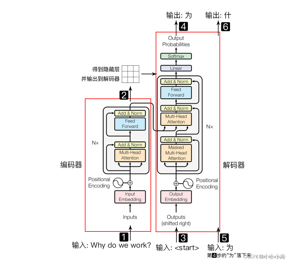
原理：https://blog.csdn.net/weixin_44649780/article/details/126808881?spm=1001.2014.3001.5501

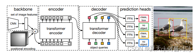
图2： DETR使用一个传统的CNN主干来学习一个输入图像的二维表示。该模型对其进行扁平化处理，并在将其传递给变换器编码器之前用位置编码进行补充。将其传递给一个transformer编码器。然后，transformer解码器将学习到的少量位置嵌入作为输入。我们称其为对象查询，并在解码器中输入少量固定数量的位置嵌入。另外还关注编码器的输出。我们将解码器的每个输出嵌入传递给一个共享的前馈网络（FFN），该网络预测一个检测（类别和边界框）或 "无物体 "类。

主干网络。从初始图像Ximg∈R 3×H0×W0（有3个色通道)，一个传统的CNN骨干网会生成一个较低分辨率的激活图f∈R C×H×W。我们使用的典型值是C = 2048，H, W =H0/32 ,W0/32 .

Transformer编码器。编码器希望有一个序列作为输入，因此我们将z0的空间维度折叠成一个维度，从而得到一个d×HW的特征图。每个编码器层都有一个标准的结构，由一个多头的自我注意模块和一个前馈网络（FFN）。
encoder的输入包含三部分，

（1）由图像生成的序列：src (HW, N , 256),

（2）掩码信息：mask (N, HW),

（3）位置信息：pos_embed(HW, N ,256)
参考：https://blog.csdn.net/sazass/article/details/118329320

Transformer解码器。解码器遵循转化器的标准结构。transformer的标准结构，使用多头的自和
编码器-解码器注意机制。与原始转化器的区别是，我们的模型在每个解码器层对N个对象进行并行解码。而Vaswani等人[47]使用一个自回归模型(autoregressive model)，每次预测输出的顺序一次预测一个元素。我们请不熟悉这些概念的读者参考补充材料。考补充由于解码器也是互换不变的。N个输入嵌入必须是不同的，以产生不同的结果。这些输入嵌入是学习到的位置编码，我们将其称为对象查询。与编码器类似，我们将它们添加到每个注意力层的输入中。N个对象查询被解码器转化为输出嵌入。然后，它们被一个前馈网络独立地解码为盒子坐标和类别标签。一个前馈网络（在下一小节中描述），产生N个最终的预测。使用自我和编码器-解码器对这些嵌入的关注。该模型使用成对的关系对所有物体进行全局推理之间的关系，同时能够使用整个图像作为背景。

归纳预测前馈网络（FFNs）。最终的预测是由一个具有ReLU激活函数和隐藏维度d的3层感知器和一个线性投影层计算的。FFN预测的是归一化的中心坐标、预测框的高度和宽度（相对于输入图像），而线性层则使用softmax函数预测类别标签。由于我们预测的是一个固定大小的N个边界框，而N通常比图像中感兴趣的物体的实际数量要大得多，所以一个额外的特殊类标签∅被用来表示在一个槽内没有检测到任何物体。这个类别扮演着与标准物体检测方法中的 "背景 "类类似的角色。

辅助解码损失。我们发现在训练过程中使用辅助损失[1]对解码器很有帮助，特别是帮助模型输出每个类别的正确数量的对象。我们在每个解码层之后添加预测的FFN和匈牙利损失。解码器层之后。所有的预测FFNs共享它们的参数。我们使用一个额外的共享层规范来规范来自不同解码层的预测FFN的输入。
流程：主干网络（resnet50）------位置编码器-----transformer编码器-----transformer解码器----FFN预测—计算loss

self.self_attn = nn.MultiheadAttention(d_model, nhead, dropout=dropout)    ##256,8
_hidden_dim=256
_num_queries=100
self.query_embed = nn.Embedding(num_queries, _hidden_dim)
features, pos = self.backbone(samples)    ##src是backbone的输出；pos是backbone+位置编码后的输出
src, mask = features[-1].decompose()
hs = self.transformer(self.input_proj(src), mask, self.query_embed.weight, pos[-1])[0]
encoder的forward：q = k = self.with_pos_embed(src, pos)src2 = self.self_attn(q, k, value=src, attn_mask=src_mask,key_padding_mask=src_key_padding_mask)[0]src = src + self.dropout1(src2)src = self.norm1(src)src2 = self.linear2(self.dropout(self.activation(self.linear1(src))))src = src + self.dropout2(src2)src = self.norm2(src)return src
transformer的forward：memory = self.encoder(src, src_key_padding_mask=mask, pos=pos_embed)hs = self.decoder(tgt, memory, memory_key_padding_mask=mask,pos=pos_embed, query_pos=query_embed)
class TransformerDecoderLayer(nn.Module):def __init__(self, d_model, nhead, dim_feedforward=2048, dropout=0.1,activation="relu", normalize_before=False):super().__init__()self.self_attn = nn.MultiheadAttention(d_model, nhead, dropout=dropout)self.multihead_attn = nn.MultiheadAttention(d_model, nhead, dropout=dropout)# Implementation of Feedforward modelself.linear1 = nn.Linear(d_model, dim_feedforward)self.dropout = nn.Dropout(dropout)self.linear2 = nn.Linear(dim_feedforward, d_model)self.norm1 = nn.LayerNorm(d_model)self.norm2 = nn.LayerNorm(d_model)self.norm3 = nn.LayerNorm(d_model)self.dropout1 = nn.Dropout(dropout)self.dropout2 = nn.Dropout(dropout)self.dropout3 = nn.Dropout(dropout)self.activation = _get_activation_fn(activation)self.normalize_before = normalize_before

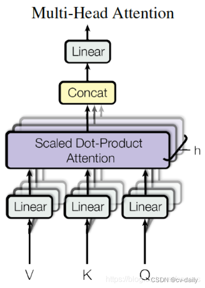
Q 的 shape 就是 n*dmodel， K、V 也是一样
out = {‘pred_logits’: outputs_class[-1], ‘pred_boxes’: outputs_coord[-1]}
if self.aux_loss:
out[‘aux_outputs’] = self._set_aux_loss(outputs_class, outputs_coord)

batchx3x768x992-----batchx2048x24x31------卷积得到src=batchx_hidden_dimx24x31-----变换到744xbatchx _hidden_dim（q，k，v的维度）-----编码完还是744xbatchx _hidden_dim-----解码得到6x2x100x256-----分别计算类别全连接outputs_class：6x2x100x（num_cls+1）和位置MLP层outputs_coord：6x2x100x4

out = {'pred_logits': outputs_class[-1], 'pred_boxes': outputs_coord[-1]}  ##pred_logits是（2,100,6），pred_boxes是（2,100,4）if self.aux_loss:out['aux_outputs'] = self._set_aux_loss(outputs_class, outputs_coord)

位置编码器参考：https://blog.csdn.net/weixin_44649780/article/details/127162890
作用：对backbone输出的二维特征添加上位置信息（b,c,h/32,w/32）.
DETR中提供了两种编码方式，一种是正弦编码（PositionEmbeddingSine），一种是可以学习的编码(PositionEmbeddingLearned)，默认为正弦编码。
对x或y，计算奇数位置的正弦，计算偶数位置的余弦，然后将pos_x和pos_y拼接起来得到一个NHWD的数组，再经过permute(0,3,1,2)，形状变为NDHW，其中D等于hidden_dim。这个hidden_dim是Transformer输入向量的维度，在实现上，要等于CNN backbone输出的特征图的维度。所以pos code和CNN输出特征的形状是完全一样的。

使用：https://zhuanlan.zhihu.com/p/566438910
1.数据集yolo转coco
“”"
YOLO 格式的数据集转化为 COCO 格式的数据集
–root_dir 输入根路径
–save_path 保存文件的名字(没有random_split时使用)
–random_split 有则会随机划分数据集，然后再分别保存为3个文件。
–split_by_file 按照 ./train.txt ./val.txt ./test.txt 来对数据集进行划分。

"""import os
import cv2
import json
from tqdm import tqdm
from sklearn.model_selection import train_test_split
import argparseparser = argparse.ArgumentParser()
parser.add_argument('--root_dir', default='./val', type=str,help="root path of images and labels, include ./images and ./labels and classes.txt")
parser.add_argument('--save_path', type=str, default='./val.json',help="if not split the dataset, give a path to a json file")
parser.add_argument('--random_split', action='store_true', help="random split the dataset, default ratio is 8:1:1")
parser.add_argument('--split_by_file', action='store_true',help="define how to split the dataset, include ./train.txt ./val.txt ./test.txt ")arg = parser.parse_args()def train_test_val_split_random(img_paths, ratio_train=0.8, ratio_test=0.1, ratio_val=0.1):# 这里可以修改数据集划分的比例。assert int(ratio_train + ratio_test + ratio_val) == 1train_img, middle_img = train_test_split(img_paths, test_size=1 - ratio_train, random_state=233)ratio = ratio_val / (1 - ratio_train)val_img, test_img = train_test_split(middle_img, test_size=ratio, random_state=233)print("NUMS of train:val:test = {}:{}:{}".format(len(train_img), len(val_img), len(test_img)))return train_img, val_img, test_imgdef train_test_val_split_by_files(img_paths, root_dir):# 根据文件 train.txt, val.txt, test.txt（里面写的都是对应集合的图片名字） 来定义训练集、验证集和测试集phases = ['train', 'val', 'test']img_split = []for p in phases:define_path = os.path.join(root_dir, f'{p}.txt')print(f'Read {p} dataset definition from {define_path}')assert os.path.exists(define_path)with open(define_path, 'r') as f:img_paths = f.readlines()# img_paths = [os.path.split(img_path.strip())[1] for img_path in img_paths]  # NOTE 取消这句备注可以读取绝对地址。img_split.append(img_paths)return img_split[0], img_split[1], img_split[2]def yolo2coco(arg):root_path = arg.root_dirprint("Loading data from ", root_path)assert os.path.exists(root_path)originLabelsDir = os.path.join(root_path, 'labels')originImagesDir = os.path.join(root_path, 'images')with open(os.path.join(root_path, 'classes.txt')) as f:classes = f.read().strip().split()# images dir nameindexes = os.listdir(originImagesDir)if arg.random_split or arg.split_by_file:# 用于保存所有数据的图片信息和标注信息train_dataset = {'categories': [], 'annotations': [], 'images': []}val_dataset = {'categories': [], 'annotations': [], 'images': []}test_dataset = {'categories': [], 'annotations': [], 'images': []}# 建立类别标签和数字id的对应关系, 类别id从0开始。for i, cls in enumerate(classes, 0):train_dataset['categories'].append({'id': i, 'name': cls, 'supercategory': 'mark'})val_dataset['categories'].append({'id': i, 'name': cls, 'supercategory': 'mark'})test_dataset['categories'].append({'id': i, 'name': cls, 'supercategory': 'mark'})if arg.random_split:print("spliting mode: random split")train_img, val_img, test_img = train_test_val_split_random(indexes, 0.8, 0.1, 0.1)elif arg.split_by_file:print("spliting mode: split by files")train_img, val_img, test_img = train_test_val_split_by_files(indexes, root_path)else:dataset = {'categories': [], 'annotations': [], 'images': []}for i, cls in enumerate(classes, 0):dataset['categories'].append({'id': i, 'name': cls, 'supercategory': 'mark'})# 标注的idann_id_cnt = 0for k, index in enumerate(tqdm(indexes)):# 支持 png jpg 格式的图片。txtFile = index.replace('images', 'txt').replace('.jpg', '.txt').replace('.png', '.txt')# 读取图像的宽和高im = cv2.imread(os.path.join(root_path, 'images/') + index)height, width, _ = im.shapeif arg.random_split or arg.split_by_file:# 切换dataset的引用对象，从而划分数据集if index in train_img:dataset = train_datasetelif index in val_img:dataset = val_datasetelif index in test_img:dataset = test_dataset# 添加图像的信息dataset['images'].append({'file_name': index,'id': k,'width': width,'height': height})if not os.path.exists(os.path.join(originLabelsDir, txtFile)):# 如没标签，跳过，只保留图片信息。continuewith open(os.path.join(originLabelsDir, txtFile), 'r') as fr:labelList = fr.readlines()for label in labelList:label = label.strip().split()x = float(label[1])y = float(label[2])w = float(label[3])h = float(label[4])# convert x,y,w,h to x1,y1,x2,y2H, W, _ = im.shapex1 = (x - w / 2) * Wy1 = (y - h / 2) * Hx2 = (x + w / 2) * Wy2 = (y + h / 2) * H# 标签序号从0开始计算, coco2017数据集标号混乱，不管它了。cls_id = int(label[0])width = max(0, x2 - x1)height = max(0, y2 - y1)dataset['annotations'].append({'area': width * height,'bbox': [x1, y1, width, height],'category_id': cls_id,'id': ann_id_cnt,'image_id': k,'iscrowd': 0,# mask, 矩形是从左上角点按顺时针的四个顶点'segmentation': [[x1, y1, x2, y1, x2, y2, x1, y2]]})ann_id_cnt += 1# 保存结果folder = os.path.join(root_path, 'annotations')if not os.path.exists(folder):os.makedirs(folder)if arg.random_split or arg.split_by_file:for phase in ['train', 'val', 'test']:json_name = os.path.join(root_path, 'annotations/{}.json'.format(phase))with open(json_name, 'w') as f:if phase == 'train':json.dump(train_dataset, f)elif phase == 'val':json.dump(val_dataset, f)elif phase == 'test':json.dump(test_dataset, f)print('Save annotation to {}'.format(json_name))else:json_name = os.path.join(root_path, 'annotations/{}'.format(arg.save_path))with open(json_name, 'w') as f:json.dump(dataset, f)print('Save annotation to {}'.format(json_name))if __name__ == "__main__":yolo2coco(arg)

2.下载代码

git clone https://github.com/facebookresearch/detr.git

然后修改几个东西

首先去官方github上下载权重，修改需训练权重文件，新建一个change.py

注意num_class要是类别数加1，例如你是2类，就改为3

import torch
pretrained_weights = torch.load(‘detr-r50-e632da11.pth’)

num_class = 3 # 这里是你自己数据集的类别数量 + 1

pretrained_weights["model"]["class_embed.weight"].resize_(num_class+1, 256)
pretrained_weights["model"]["class_embed.bias"].resize_(num_class+1)
torch.save(pretrained_weights, "detr-r50_%d.pth"%num_class)

然后执行 python change.py 得到 detr-r50-3.pth 这个权重

接下来修改./models/detr.py

305行的 num_classes = 类别数 + 1

如果就可以训练了

参数想改哪个就改哪个
3.训练

def build_backbone(args):position_embedding = build_position_encoding(args)  ##正余弦位置编码/train_backbone = args.lr_backbone > 0return_interm_layers = args.masksbackbone = Backbone(args.backbone, train_backbone, return_interm_layers, args.dilation)   ##resnet50model = Joiner(backbone, position_embedding)model.num_channels = backbone.num_channelsreturn model

python main.py --dataset_file "coco" --coco_path coco_data --epochs 100 --lr=1e-4 --batch_size=2 --num_workers=4 --output_dir="outputs" --resume="detr-r50_3.pth"

4.代码解读
模型构建：

def build(args):num_classes = 5if args.dataset_file == "coco_panoptic":# for panoptic, we just add a num_classes that is large enough to hold# max_obj_id + 1, but the exact value doesn't really matternum_classes = 250device = torch.device(args.device)backbone = build_backbone(args)transformer = build_transformer(args)model = DETR(backbone,transformer,num_classes=num_classes,num_queries=args.num_queries,aux_loss=args.aux_loss,)if args.masks:model = DETRsegm(model, freeze_detr=(args.frozen_weights is not None))matcher = build_matcher(args)weight_dict = {'loss_ce': 1, 'loss_bbox': args.bbox_loss_coef}weight_dict['loss_giou'] = args.giou_loss_coefif args.masks:weight_dict["loss_mask"] = args.mask_loss_coefweight_dict["loss_dice"] = args.dice_loss_coef# TODO this is a hackif args.aux_loss:aux_weight_dict = {}for i in range(args.dec_layers - 1):aux_weight_dict.update({k + f'_{i}': v for k, v in weight_dict.items()})weight_dict.update(aux_weight_dict)losses = ['labels', 'boxes', 'cardinality']if args.masks:losses += ["masks"]criterion = SetCriterion(num_classes, matcher=matcher, weight_dict=weight_dict,eos_coef=args.eos_coef, losses=losses)criterion.to(device)postprocessors = {'bbox': PostProcess()}if args.masks:postprocessors['segm'] = PostProcessSegm()if args.dataset_file == "coco_panoptic":is_thing_map = {i: i <= 90 for i in range(201)}postprocessors["panoptic"] = PostProcessPanoptic(is_thing_map, threshold=0.85)return model, criterion, postprocessors

匈牙利匹配

class HungarianMatcher(nn.Module):def __init__(self, cost_class: float = 1, cost_bbox: float = 1, cost_giou: float = 1):super().__init__()self.cost_class = cost_classself.cost_bbox = cost_bboxself.cost_giou = cost_giouassert cost_class != 0 or cost_bbox != 0 or cost_giou != 0, "all costs cant be 0"@torch.no_grad()def forward(self, outputs, targets):bs, num_queries = outputs["pred_logits"].shape[:2]# We flatten to compute the cost matrices in a batchout_prob = outputs["pred_logits"].flatten(0, 1).softmax(-1)  # [batch_size * num_queries, num_classes]out_bbox = outputs["pred_boxes"].flatten(0, 1)  # [batch_size * num_queries, 4]# Also concat the target labels and boxestgt_ids = torch.cat([v["labels"] for v in targets])tgt_bbox = torch.cat([v["boxes"] for v in targets])cost_class = -out_prob[:, tgt_ids]  # tgt_ids是[1,2,1,0，...]，该batch中所有的目标类别# Compute the L1 cost between boxescost_bbox = torch.cdist(out_bbox, tgt_bbox, p=1)# tgt_ids该batch中所有的目标的位置[总目标数，4]# Compute the giou cost betwen boxescost_giou = -generalized_box_iou(box_cxcywh_to_xyxy(out_bbox), box_cxcywh_to_xyxy(tgt_bbox))# Final cost matrixC = self.cost_bbox * cost_bbox + self.cost_class * cost_class + self.cost_giou * cost_giou     ##类别损失+bbox的l1损失+bbox的giou损失C = C.view(bs, num_queries, -1).cpu()sizes = [len(v["boxes"]) for v in targets]indices = [linear_sum_assignment(c[i]) for i, c in enumerate(C.split(sizes, -1))]return [(torch.as_tensor(i, dtype=torch.int64), torch.as_tensor(j, dtype=torch.int64)) for i, j in indices]def build_matcher(args):return HungarianMatcher(cost_class=args.set_cost_class, cost_bbox=args.set_cost_bbox, cost_giou=args.set_cost_giou)

用自己的数据集训练完，测试结果：

IoU metric: bboxAverage Precision  (AP) @[ IoU=0.50:0.95 | area=   all | maxDets=100 ] = 0.712Average Precision  (AP) @[ IoU=0.50      | area=   all | maxDets=100 ] = 0.911Average Precision  (AP) @[ IoU=0.75      | area=   all | maxDets=100 ] = 0.779Average Precision  (AP) @[ IoU=0.50:0.95 | area= small | maxDets=100 ] = 0.049Average Precision  (AP) @[ IoU=0.50:0.95 | area=medium | maxDets=100 ] = 0.443Average Precision  (AP) @[ IoU=0.50:0.95 | area= large | maxDets=100 ] = 0.752Average Recall     (AR) @[ IoU=0.50:0.95 | area=   all | maxDets=  1 ] = 0.452Average Recall     (AR) @[ IoU=0.50:0.95 | area=   all | maxDets= 10 ] = 0.814Average Recall     (AR) @[ IoU=0.50:0.95 | area=   all | maxDets=100 ] = 0.846Average Recall     (AR) @[ IoU=0.50:0.95 | area= small | maxDets=100 ] = 0.189Average Recall     (AR) @[ IoU=0.50:0.95 | area=medium | maxDets=100 ] = 0.645Average Recall     (AR) @[ IoU=0.50:0.95 | area= large | maxDets=100 ] = 0.878

比yolov5s P=0.96，R=0.90精度低一些。