【无人机】回波状态网络(ESN)在固定翼无人机非线性控制中的应用(Matlab代码实现)

💥💥💞💞欢迎来到本博客❤️❤️💥💥
🏆博主优势:🌞🌞🌞博客内容尽量做到思维缜密,逻辑清晰,为了方便读者。
⛳️座右铭:行百里者,半于九十。
📋📋📋本文目录如下:🎁🎁🎁
目录
💥1 概述
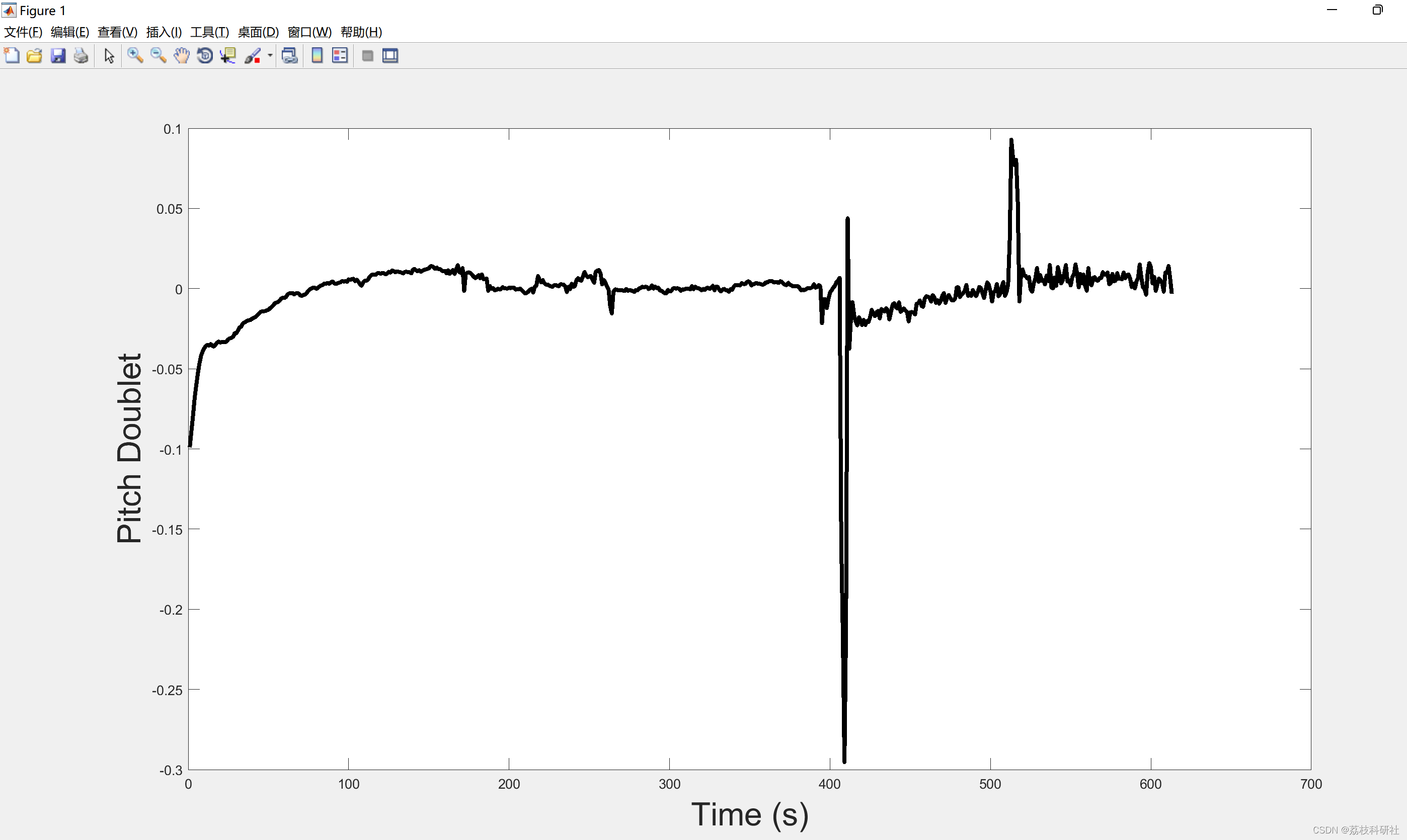
📚2 运行结果
🎉3 参考文献
🌈4 Matlab代码实现

💥1 概述
无人机为执行各种军事和民用任务提供了平台。这包括情报、监视和侦察( ISR )、战场损伤评估和部队保护等军事应用。民用应用包括遥感、科学研究、搜救任务、边境巡逻、受灾地区监测、航空摄影、航空测绘岩土工程、植被生长分析、农作物除尘、精准农业、地形变化评估等。无人机产业是航天工业中发展最快的部门,民用无人机的使用也在显著增长。据估计,在未来十年中,无人机的支出将从目前全世界每年52亿美元的支出翻一番。一旦技术成熟,将无人机集成到国家空间系统( NAS )中,本文是为无人机开发自适应飞行控制器。包括多层感知器( MLP )和回声状态网络( ESN )。MLP用于离线模型,而ESN用于在线模型。MLP将成为焦点,因为它的自适应和循环行为允许它自然地坚持经典控制律,并完成反馈回路。ESN采用有监督的时序方法进行机器学习。这使得它成为解决诸如飞行控制器等动态系统问题的备选方案。MLP将主要用于误差校正。ESN是稀疏连接的,隐藏层有12个神经元,具有单一的输入和输出信号。隐藏层充当一个储液器,因为它表现出电流已知的40 %泄漏率。详细文章讲解见第4部分。
📚2 运行结果

部分代码:
% NSF Twin Engine Doublet Data
clc
clear
% Read log file
Data = xlsread('Fri May 24 14-54-11 2013e.xlsx');
% Read in time (ms)
t = Data(:,1)-27081;
% Convert milli seconds to seconds
tsec = t./1000;
% Convert seconds to minutes
tmin = tsec./60;
% Determine the point at which 1 Hz recording to 10 Hz recording
tdiff = diff(tsec);
%Change time set to only contain 10 Hz data
tsec2 = tsec(829:4557);
%Roll Rate
P = Data(:,32).*(180/pi());
Pflight = P(829:4557);
% Pitch Rate
Q = Data(:,33).*(180/pi());
Qflight = Q(829:4557);
% Yaw Rate
R = Data(:,34).*(180/pi());
Rflight = R(829:4557);
% Roll
Roll = Data(:,38).*(180/pi());
Roll_flight = Roll(829:4557);
% Pitch
Pitch = Data(:,39).*(180/pi());
Pitch_flight = Pitch(829:4557);
% Yaw
Yaw = Data(:,40).*(180/pi());
Yaw_flight = Yaw(829:4557);
% Acknowledgement Ratio
AckRatio = Data(:,49);
AckRatio_flight = AckRatio(829:4557);
% RSSI
RSSI = Data(:,50);
RSSI_flight = RSSI(829:4557);
% Surface 0
% Aileron
Surface0 = Data(:,51);
Sur0_flight = Surface0(829:4557).*(180/pi());
% Looking for constant surface deflection
Aileron1_diff = diff(Sur0_flight);
% Surface 1
% Elevator
Surface1 = Data(:,52).*(180/pi());
Sur1_flight = Surface1(829:4557);
% Looking for constant surface deflection
Elevator1_diff = diff(Sur1_flight);
% Surface 2
% Throttle
Surface2 = Data(:,53);
Sur2_flight = Surface2(829:4557);
% Looking for constant surface deflection
Throttle1_diff = diff(Sur2_flight);
% Surface 3
Surface3 = Data(:,54).*(180/pi());
Sur3_flight = Surface3(829:4557);
% Looking for constant surface deflection
Sur3_diff = diff(Sur3_flight);
% Surface 4
Surface4 = Data(:,55).*(180/pi());
Sur4_flight = Surface4(829:4557);
% Looking for constant surface deflection
Sur4_diff = diff(Sur3_flight);
% Surface 5
% Aileron
Surface5 = Data(:,56).*(180/pi());
Sur5_flight = Surface5(829:4557);
% Looking for constant surface deflection
Aileron2_diff = diff(Sur5_flight);
% Surface 6
% Elevator
Surface6 = Data(:,57).*(180/pi());
Sur6_flight = Surface6(829:4557);
% Looking for constant surface deflection
Elevator2_diff = diff(Sur6_flight);
% Surface 7
% Throttle
Surface7 = Data(:,58);
Sur7_flight = Surface7(829:4557);
% Looking for constant surface deflection
Throttle2_diff = diff(Sur7_flight);
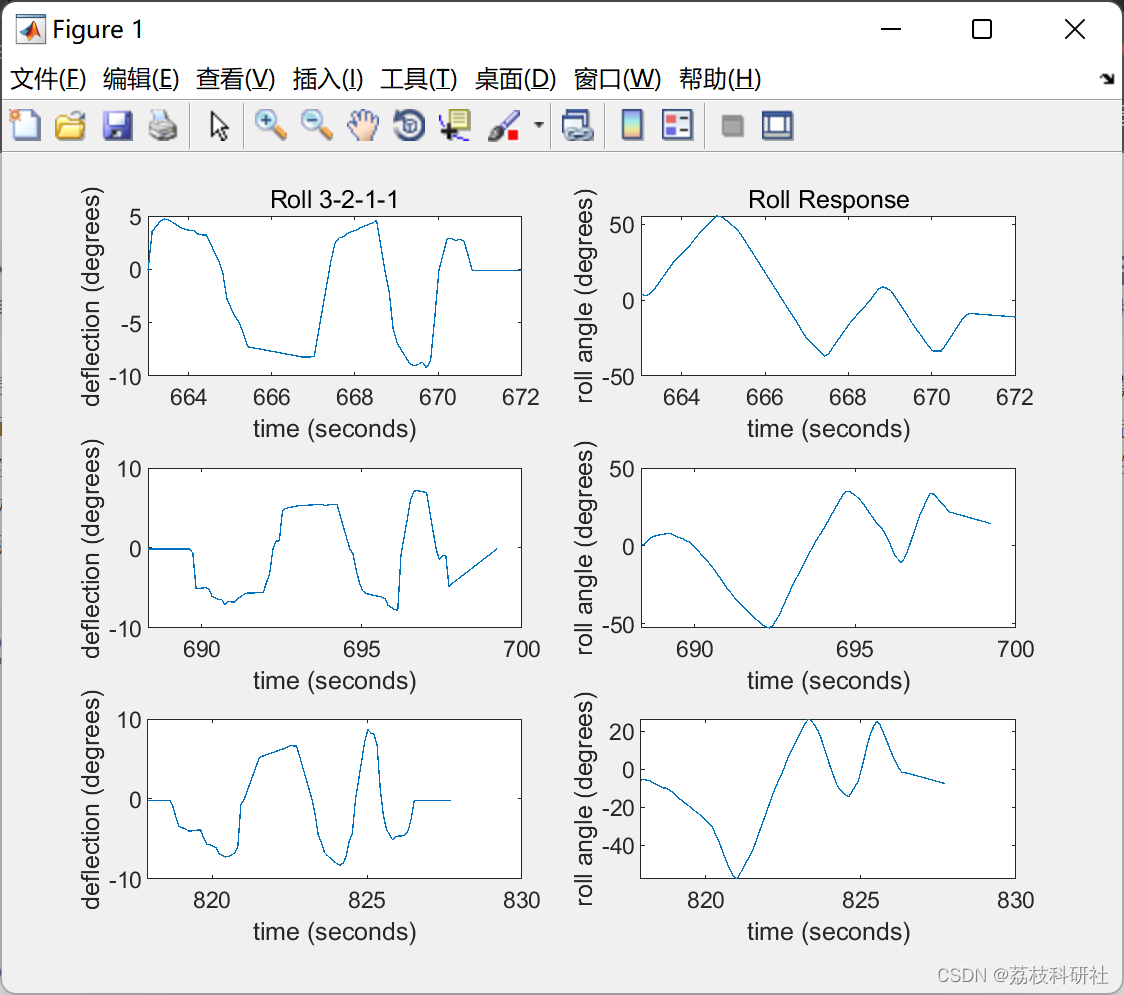
% Roll 3-2-1-1
% 1567-1624 No Elevator Movement
subplot(3,2,1)
plot(tsec2(1567:1624),Sur0_flight(1567:1624))
xlabel('time (seconds)')
ylabel('deflection (degrees)')
title('Roll 3-2-1-1')
subplot(3,2,2)
plot(tsec2(1567:1624),Roll_flight(1567:1624))
title('Roll Response')
xlabel('time (seconds)')
ylabel('roll angle (degrees)')
% 1733-1805 No Elevator Movement
subplot(3,2,3)
plot(tsec2(1733:1805),Sur0_flight(1733:1805))
xlabel('time (seconds)')
ylabel('deflection (degrees)')
subplot(3,2,4)
plot(tsec2(1733:1805),Roll_flight(1733:1805))
xlabel('time (seconds)')
ylabel('roll angle (degrees)')
% 2563-2628 No Elevator Movement
subplot(3,2,5)
plot(tsec2(2563:2628),Sur0_flight(2563:2628))
xlabel('time (seconds)')
ylabel('deflection (degrees)')
subplot(3,2,6)
plot(tsec2(2563:2628),Roll_flight(2563:2628))
xlabel('time (seconds)')
ylabel('roll angle (degrees)')
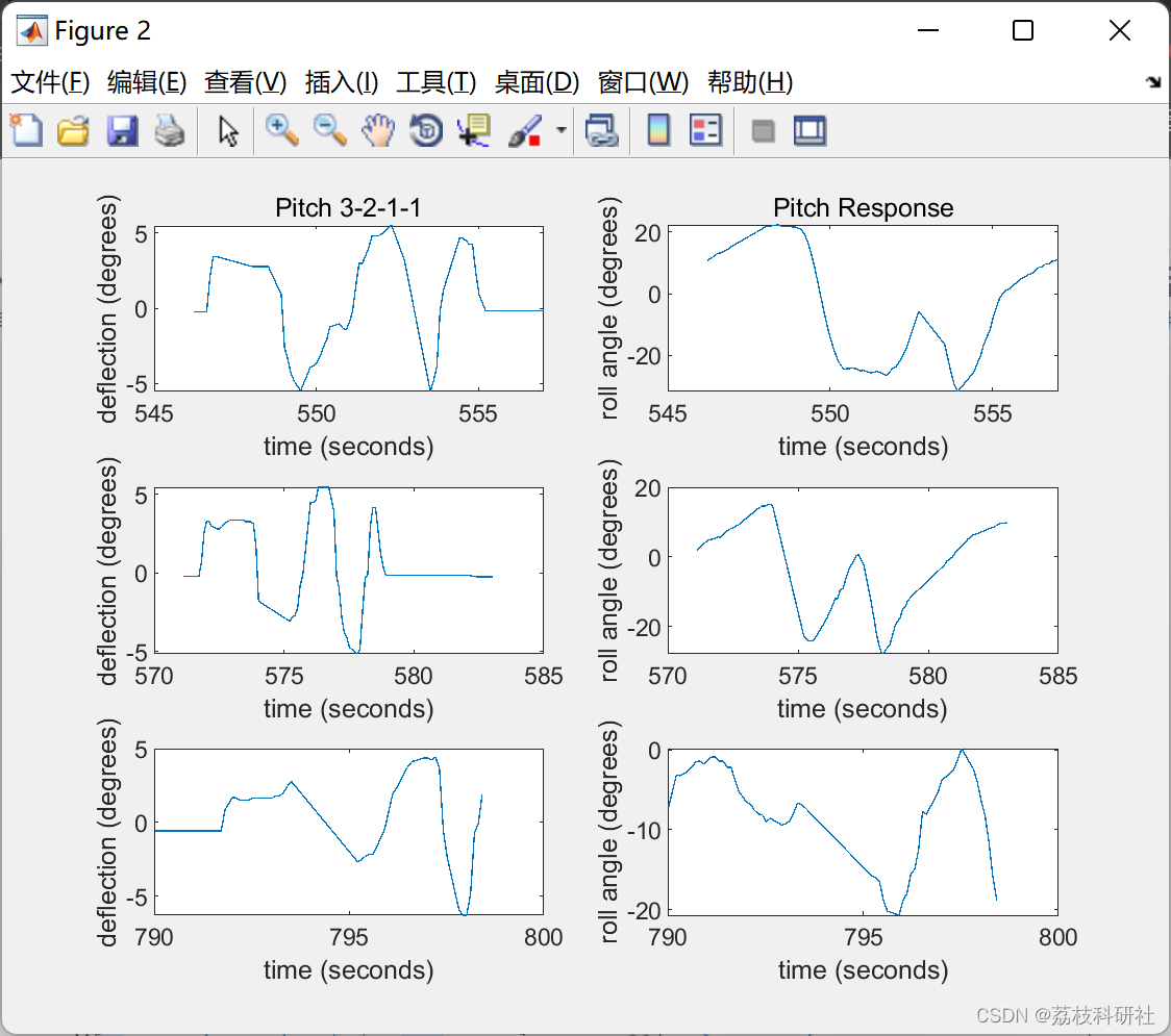
% Pitch 3-2-1-1
% 908 - 980 No Aileron Movement
figure
subplot(3,2,1)
plot(tsec2(908:980),Sur1_flight(908:980))
xlabel('time (seconds)')
ylabel('deflection (degrees)')
title('Pitch 3-2-1-1')
subplot(3,2,2)
plot(tsec2(908:980),Pitch_flight(908:980))
title('Pitch Response')
xlabel('time (seconds)')
ylabel('roll angle (degrees)')
% 1068 - 1148 No Aileron Movement
subplot(3,2,3)
plot(tsec2(1068:1148),Sur1_flight(1068:1148))
xlabel('time (seconds)')
ylabel('deflection (degrees)')
subplot(3,2,4)
plot(tsec2(1068:1148),Pitch_flight(1068:1148))
xlabel('time (seconds)')
ylabel('roll angle (degrees)')
% 2380 - 2437 No Aileron Movement
subplot(3,2,5)
plot(tsec2(2380:2437),Sur1_flight(2380:2437))
xlabel('time (seconds)')
ylabel('deflection (degrees)')
subplot(3,2,6)
plot(tsec2(2380:2437),Roll_flight(2380:2437))
xlabel('time (seconds)')
ylabel('roll angle (degrees)')
figure (3), subplot(2,1,1),plot(tsec2(1567:1624),Sur0_flight(1567:1624),'k-','linewidth',3)
grid
ylabel('Aileron (deg)','fontsize',25)
title('Roll Doublet','fontsize',25),set(gca,'fontsize',25)
subplot(2,1,2),plot(tsec2(1567:1624),Roll_flight(1567:1624),'k-','linewidth',3)
ylabel('Roll Angle (deg)','fontsize',25),grid,set(gca,'fontsize',25)
xlabel('Time (sec)')
🎉3 参考文献
部分理论来源于网络,如有侵权请联系删除。