【CS224W】(task12)GAT GNN training tips

note
- GAT使用attention对线性转换后的节点进行加权求和:利用自身节点的特征向量分别和邻居节点的特征向量,进行内积计算score。
- 异质图的消息传递和聚合:hv(l+1)=σ(∑r∈R∑u∈Nvr1cv,rWr(l)hu(l)+W0(l)hv(l))\\mathbf{h}_v^{(l+1)}=\\sigma\\left(\\sum_{r \\in R} \\sum_{u \\in N_v^r} \\frac{1}{c_{v, r}} \\mathbf{W}_r^{(l)} \\mathbf{h}_u^{(l)}+\\mathbf{W}_0^{(l)} \\mathbf{h}_v^{(l)}\\right) hv(l+1)=σr∈R∑u∈Nvr∑cv,r1Wr(l)hu(l)+W0(l)hv(l)
文章目录
- note
- 一、GAT model
- 二、GNN模型训练要点
-
- 1. Graph Manipulation
- 2. GNN training
-
- (1)Node-level
- (2)Edge-level
- (3)Graph-level
- 3. Issue of Global pooling
-
- (1)Global pooling的毛病
- (2)DidffPool 社群分层池化:
- 三、GNN training tips
-
- 3.1 Spliting Graphs is special
- 3.2 异质图 Heterogeneous graph
- 附:时间安排
- Reference
一、GAT model
图注意神经网络(GAT)来源于论文 Graph Attention Networks。其数学定义为,
xi′=αi,iΘxi+∑j∈N(i)αi,jΘxj,\\mathbf{x}^{\\prime}_i = \\alpha_{i,i}\\mathbf{\\Theta}\\mathbf{x}_{i} + \\sum_{j \\in \\mathcal{N}(i)} \\alpha_{i,j}\\mathbf{\\Theta}\\mathbf{x}_{j}, xi′=αi,iΘxi+j∈N(i)∑αi,jΘxj,
GAT和所有的attention mechanism一样,GAT的计算也分为两步走:
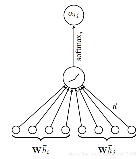
(1)计算注意力系数(attention coefficient):(下图来自《GRAPH ATTENTION NETWORKS》)
其中注意力系数αi,j\\alpha_{i,j}αi,j的计算方法为,
αi,j=exp(LeakyReLU(a⊤[Θxi∥Θxj]))∑k∈N(i)∪{i}exp(LeakyReLU(a⊤[Θxi∥Θxk])).\\alpha_{i,j} = \\frac{ \\exp\\left(\\mathrm{LeakyReLU}\\left(\\mathbf{a}^{\\top} [\\mathbf{\\Theta}\\mathbf{x}_i \\, \\Vert \\, \\mathbf{\\Theta}\\mathbf{x}_j] \\right)\\right)} {\\sum_{k \\in \\mathcal{N}(i) \\cup \\{ i \\}} \\exp\\left(\\mathrm{LeakyReLU}\\left(\\mathbf{a}^{\\top} [\\mathbf{\\Theta}\\mathbf{x}_i \\, \\Vert \\, \\mathbf{\\Theta}\\mathbf{x}_k] \\right)\\right)}. αi,j=∑k∈N(i)∪{i}exp(LeakyReLU(a⊤[Θxi∥Θxk]))exp(LeakyReLU(a⊤[Θxi∥Θxj])).
(2)加权求和(aggregate):根据(1)的系数,把特征加权求和(aggregate)hv(l)=σ(∑u∈N(v)αvuW(l)hu(l−1))\\mathbf{h}_v^{(l)}=\\sigma\\left(\\sum_{u \\in N(v)} \\alpha_{v u} \\mathbf{W}^{(l)} \\mathbf{h}_u^{(l-1)}\\right) hv(l)=σu∈N(v)∑αvuW(l)hu(l−1)

二、GNN模型训练要点
1. Graph Manipulation

- feature manipulation:feature augmentation, such as we can use cycle count as augmented node features
- struture manipulation:
- sparse graph: add virtual nodes or edges
- dense graph: sample neighbors when doing message passing
- large graph: sample subgraphs to compute embeddings
2. GNN training
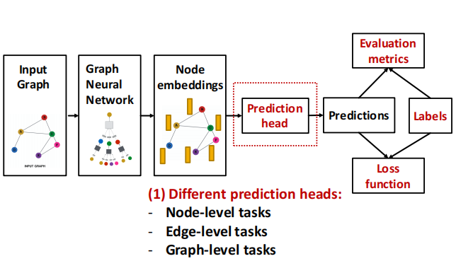
(1)Node-level
- After GNN computation, we have ddd-dim node
embeddings: {hv(L)∈Rd,∀v∈G}\\text { embeddings: }\\left\\{\\mathbf{h}_v^{(L)} \\in \\mathbb{R}^d, \\forall v \\in G\\right\\} embeddings: {hv(L)∈Rd,∀v∈G} - such as k-way prediction:
- y^v=Headnode (hv(L))=W(H)hv(L)\\widehat{\\boldsymbol{y}}_v=\\operatorname{Head}_{\\text {node }}\\left(\\mathbf{h}_v^{(L)}\\right)=\\mathbf{W}^{(H)} \\mathbf{h}_v^{(L)}yv=Headnode (hv(L))=W(H)hv(L)
- W(H)∈Rk∗d\\mathbf{W}^{(H)} \\in \\mathbb{R}^{k * d}W(H)∈Rk∗d : We map node embeddings from hv(L)∈Rd\\mathbf{h}_v^{(L)} \\in \\mathbb{R}^dhv(L)∈Rd to y^v∈Rk\\widehat{y}_v \\in \\mathbb{R}^kyv∈Rk
- compute the loss
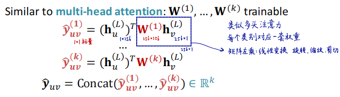
(2)Edge-level
- use pairs of node embeddings
- such as k-way prediction:y^uv=Headedge (hu(L),hv(L))\\widehat{\\boldsymbol{y}}_{u v}=\\operatorname{Head}_{\\text {edge }}\\left(\\mathbf{h}_u^{(L)}, \\mathbf{h}_v^{(L)}\\right)yuv=Headedge (hu(L),hv(L))
- Concatenation + Linear:y^uv=Linear(Concat(hu(L),hv(L)))\\hat{\\boldsymbol{y}}_{u v}=\\operatorname{Linear}\\left(\\operatorname{Concat}\\left(\\mathbf{h}_u^{(L)}, \\mathbf{h}_v^{(L)}\\right)\\right)y^uv=Linear(Concat(hu(L),hv(L))),and Linear\\operatorname{Linear}Linear can map 2d-dim embeddings to k-dim embeddings
- Dot product :y^uv=(hu(L))Thv(L)\\hat{\\boldsymbol{y}}_{\\boldsymbol{u} v}=\\left(\\mathbf{h}_u^{(L)}\\right)^T \\mathbf{h}_v^{(L)}y^uv=(hu(L))Thv(L)
- this approach only applies to 1-way prediction(预测边是否存在)
- k-way prediction:
(3)Graph-level
- use all the node embeddings in our graph
- such as k-way prediction:y^G=Headgraph({hv(L)∈Rd,∀v∈G})\\widehat{\\boldsymbol{y}}_G=\\operatorname{Head}_{\\operatorname{graph}}\\left(\\left\\{\\mathbf{h}_v^{(L)} \\in \\mathbb{R}^d, \\forall v \\in G\\right\\}\\right)yG=Headgraph({hv(L)∈Rd,∀v∈G})
- Headgraph\\operatorname{Head}_{\\operatorname{graph}}Headgraph ≈ AGG(`) in a GNN layer
- Gloal pooling:use Gloal mean or max or sum pooling instead of Headgraph\\operatorname{Head}_{\\operatorname{graph}}Headgraph
3. Issue of Global pooling
(1)Global pooling的毛病
- Useing global pooling over a large graph will lose information
- toy example(1-dim node embeddings):
- Node embeddings for G1:{−1,−2,0,1,2}G_1:\\{-1,-2,0,1,2\\}G1:{−1,−2,0,1,2}, global sum pooling ans:0
- Node embeddings for G2:{−10,−20,0,10,20}G_2:\\{-10,-20,0,10,20\\}G2:{−10,−20,0,10,20},global sum pooling ans:0
- 特点:只看均值,不看方差
- so we can use hierarchical pooling 分层池化
- toy example:We will aggregate via ReLU(Sum(⋅))\\operatorname{ReLU}(\\operatorname{Sum}(\\cdot))ReLU(Sum(⋅))
- We first separately aggregate the first 2 nodes and last 3 nodes;Then we aggregate again to make the final prediction
- G1G_1G1 node embeddings: {−1,−2,0,1,2}\\{-1,-2,0,1,2\\}{−1,−2,0,1,2}
- Round 1: y^a=ReLU(Sum({−1,−2}))=0,y^b=\\hat{y}_a=\\operatorname{ReLU}(\\operatorname{Sum}(\\{-1,-2\\}))=0, \\hat{y}_b=y^a=ReLU(Sum({−1,−2}))=0,y^b=
ReLU(Sum({0,1,2}))=3\\quad \\operatorname{ReLU}(\\operatorname{Sum}(\\{0,1,2\\}))=3ReLU(Sum({0,1,2}))=3 - Round 2: y^G=ReLU(Sum({ya,yb}))=3\\operatorname{Round~2:~} \\hat{y}_G=\\operatorname{ReLU}\\left(\\operatorname{Sum}\\left(\\left\\{y_a, y_b\\right\\}\\right)\\right)=3Round 2: y^G=ReLU(Sum({ya,yb}))=3
- Round 1: y^a=ReLU(Sum({−1,−2}))=0,y^b=\\hat{y}_a=\\operatorname{ReLU}(\\operatorname{Sum}(\\{-1,-2\\}))=0, \\hat{y}_b=y^a=ReLU(Sum({−1,−2}))=0,y^b=
- G2G_2G2 node embeddings: {−10,−20,0,10,20}\\{-10,-20,0,10,20\\}{−10,−20,0,10,20}
- Round 1: y^a=ReLU(Sum({−10,−20}))=0,y^b=2=\\operatorname{Round~1:~} \\hat{y}_a=\\operatorname{ReLU}(\\operatorname{Sum}(\\{-10,-20\\}))=0, \\hat{y}_b={ }^2=Round 1: y^a=ReLU(Sum({−10,−20}))=0,y^b=2=
ReLU(Sum({0,10,20}))=30\\quad \\operatorname{ReLU}(\\operatorname{Sum}(\\{0,10,20\\}))=30ReLU(Sum({0,10,20}))=30 - Round 2:y^G=ReLU(Sum({ya,yb}))=30\\operatorname{Round~2:} \\hat{y}_G=\\operatorname{ReLU}\\left(\\operatorname{Sum}\\left(\\left\\{y_a, y_b\\right\\}\\right)\\right)=30Round 2:y^G=ReLU(Sum({ya,yb}))=30
- Round 1: y^a=ReLU(Sum({−10,−20}))=0,y^b=2=\\operatorname{Round~1:~} \\hat{y}_a=\\operatorname{ReLU}(\\operatorname{Sum}(\\{-10,-20\\}))=0, \\hat{y}_b={ }^2=Round 1: y^a=ReLU(Sum({−10,−20}))=0,y^b=2=
(2)DidffPool 社群分层池化:
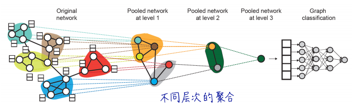
每层(将每个社群当作一层,进行社群检测)利用两个独立的GNN层(可以联合训练):
- GNN 1:计算节点embedding
- GNN 2:计算一个节点属于的社群
- 之前的图分类方法是先生成每个节点的embedding,对所有节点的embedding进行全局的pooling;而DidffPool(微分池化)通过逐渐压缩信息方式进行图分类,上一层GNN的节点进行聚类结果,作为下一层GNN的输入。
三、GNN training tips
3.1 Spliting Graphs is special
- 像图片和文本分类的样本,每个数据样本之间满足独立同分布
- 但GNN数据中不同节点可能会互相影响(消息传递)
- transductive 直推式学习:
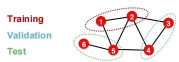
- 划分数据集时,让图结构还是能看到,可以只根据节点label进行划分。在训练和验证阶段,都是使用全图信息,如下图,利用一二节点及其label进行训练,在验证阶段也是利用整图信息,利用三四节点及其label进行验证。
- 只适合于节点or边分类任务
- inductive 归纳式学习:
- 拆分边,得到多重图
- 适合于节点or边or图分类
- transductive 直推式学习:
3.2 异质图 Heterogeneous graph
异质图比同构图多了两个属性, R、TR 、 TR、T, 其中 RRR 表示边的类型、 TTT 表示节点的类型, 最后整张图可以表示为:
G=(V,E,R,T)G=(V, E, R, T) G=(V,E,R,T)
同质图的聚合:hv(l)=σ(∑u∈N(v)W(l)hu(l−1)∣N(v)∣)\\mathbf{h}_v^{(l)}=\\sigma\\left(\\sum_{u \\in N(v)} \\mathbf{W}^{(l)} \\frac{\\mathbf{h}_u^{(l-1)}}{|N(v)|}\\right) hv(l)=σu∈N(v)∑W(l)∣N(v)∣hu(l−1)
异质图的消息传递和聚合:hv(l+1)=σ(∑r∈R∑u∈Nvr1cv,rWr(l)hu(l)+W0(l)hv(l))\\mathbf{h}_v^{(l+1)}=\\sigma\\left(\\sum_{r \\in R} \\sum_{u \\in N_v^r} \\frac{1}{c_{v, r}} \\mathbf{W}_r^{(l)} \\mathbf{h}_u^{(l)}+\\mathbf{W}_0^{(l)} \\mathbf{h}_v^{(l)}\\right) hv(l+1)=σr∈R∑u∈Nvr∑cv,r1Wr(l)hu(l)+W0(l)hv(l)
其中对于每种类型的边r,对应的邻居节点u,两节点之间传播的信息为:mu,r(l)=1cv,rWr(l)hu(l)\\mathbf{m}_{u, r}^{(l)}=\\frac{1}{c_{v, r}} \\mathbf{W}_r^{(l)} \\mathbf{h}_u^{(l)} mu,r(l)=cv,r1Wr(l)hu(l)
附:时间安排
| 任务 | 任务内容 | 截止时间 | 注意事项 |
|---|---|---|---|
| 2月11日开始 | |||
| task1 | 图机器学习导论 | 2月14日周二 | 完成 |
| task2 | 图的表示和特征工程 | 2月15、16日周四 | 完成 |
| task3 | NetworkX工具包实践 | 2月17、18日周六 | 完成 |
| task4 | 图嵌入表示 | 2月19、20日周一 | 完成 |
| task5 | deepwalk、Node2vec论文精读 | 2月21、22、23、24日周五 | 完成 |
| task6 | PageRank | 2月25、26日周日 | 完成 |
| task7 | 标签传播与节点分类 | 2月27、28日周二 | 完成 |
| task8 | 图神经网络基础 | 3月1、2日周四 | 完成 |
| task9 | 图神经网络的表示能力 | 3月3日周五 | 完成 |
| task10 | 图卷积神经网络GCN | 3月4日周六 | 完成 |
| task11 | 图神经网络GraphSAGE | 3月5日周七 | 完成 |
| task12 | 图神经网络GAT | 3月6日周一 | 完成 |
Reference
[1] https://docs.dgl.ai/en/0.8.x/generated/dgl.nn.pytorch.conv.GINConv.html?highlight=ginconv#dgl.nn.pytorch.conv.GINConv
[2] CS224W官网:https://web.stanford.edu/class/cs224w/index.html
[3] https://github.com/TommyZihao/zihao_course/tree/main/CS224W
[4] cs224w(图机器学习)2021冬季课程学习笔记18 Colab 4:异质图
[5] https://github.com/dmlc/dgl
[6] DIFFPOOL:一种图网络的分层池化方法
[7] https://relph1119.github.io/my-team-learning/#/cs224w_learning46/ext-task
[8] 【CS224W学习笔记 day09】 异质图神经网络