知识蒸馏的核心思想就是将大模型的知识传给小模型。

这里的知识通常就是模型所学的数据分布。大模型特点一般是具有非常高的精度，但可能在速度上不行，或者是不易部署，小模型通常是易部署，速度快但精度不如大模型。

因此可以将大模型视为ground truth(并不是严格意义上的，只是打比方)，然后不断缩小大小模型之间输出的差距。因此可以将大模型作为teacher，小模型为student，学生在教师的指导下学习。

从训练角度，知识蒸馏可分为离线式蒸馏和在线式蒸馏，前者是将已训练好的教师网络和学生网络之间建立关系进行蒸馏学习，后者一般是教师和学生在蒸馏的同时也在不断的自我学习。这里举个例子，你可以将你魔改后的model作为teacher，没有改进前的为student，在两者之间建立蒸馏函数，这属于离线式。而比如你将你model中的某一层作为teacher，另一层作为student，两者在建立损失函数的同时也在自我学习，这就是在线式。

从蒸馏方式，还可以分为逻辑蒸馏和特征蒸馏。前者是对模型输出的逻辑回归进行蒸馏，后者是针对模型中的特征层进行蒸馏。比如，前者主要度量两个模型输出label，后者是可以缩小两个特征层的距离。

有关离线式蒸馏可以参考我另一篇文章：分类网络知识蒸馏

本篇文章为在线蒸馏，将以Resnet为例进行代码详解，主要涉及到逻辑蒸馏和特征蒸馏。内容比较多，系好安全带，发车~

在学习本篇文章时需要各位对Resnet代码有很深的了解，这样才好学习本篇文章，有关Resnet代码的学习我这里也给准备好了：Resnet代码学习

目录

网络定义

scala缩放层

attention层

用于自蒸馏的ResNet网络

知识蒸馏训练

网络定义

与原Resnet代码不同，在这里做的几处修改。

1.Resnet第一个卷积层conv1为7x7卷积，这里改成了3x3.

# conv1与原始Resnet不同，原始Resnet为7x7卷积
self.conv1 = nn.Conv2d(3, self.inplanes, kernel_size=3, stride=1, padding=1,bias=False)

2.conv1和layer1之间的最大池化层去除。

 # 最大池化，不过在forward中没有用到
self.maxpool = nn.MaxPool2d(kernel_size=3, stride=2, padding=1)

残差块layer1~layer4代码不变，还是调用的_make_layer函数。

3.与原Resnet代码相比，这里去除了自适应池化层和全连接层。改为4个attention层以及4个缩放层(scala)。

scala缩放层

scala层主要用于特征蒸馏中的特征层缩放，代码如下(这里仅举scala1为例)。scala1由3个定义的SepConv卷积层和一个平均池化层组成。【scala2是2个SepConv+AvgP，scala3是1个SepConv+AvgP，scala4是1个AvgP】。

self.scala1 = nn.Sequential(# 输入通道64*4=256，输出通道128*4=512SepConv(  # 尺寸减半channel_in=64 * block.expansion,channel_out=128 * block.expansion),# 输入通道128*4=512， 输出通道256*4=1024SepConv(  # 尺寸减半channel_in=128 * block.expansion,channel_out=256 * block.expansion),# 输入通道256*4=1024，输出通道512*4=2048SepConv(  # 尺寸减半channel_in=256 * block.expansion,channel_out=512 * block.expansion),# 平均池化nn.AvgPool2d(4, 4))

定义的SepConv卷积代码如下：

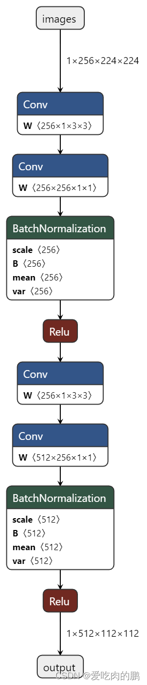
该卷积是由3x3步长为2的分组卷积、1x1卷积、BN、ReLu、3x3步长为1分组卷积、1x1卷积、BN、ReLu构成。【或者可以理解为，是由两个深度可分离卷积构成】

class SepConv(nn.Module):def __init__(self, channel_in, channel_out, kernel_size=3, stride=2, padding=1, affine=True):super(SepConv, self).__init__()self.op = nn.Sequential(# 分组卷积，这里的分组数=输入通道数，那么每个group=channel_in/channel_in=1个通道，就是每个通道进行一个卷积nn.Conv2d(channel_in, channel_in, kernel_size=kernel_size, stride=stride, padding=padding, groups=channel_in, bias=False),nn.Conv2d(channel_in, channel_in, kernel_size=1, padding=0, bias=False),# affine 设为 True 时，BatchNorm 层才会学习参数 gamma 和 beta，否则不包含这两个变量，变量名是 weight 和 bias。nn.BatchNorm2d(channel_in, affine=affine),nn.ReLU(inplace=False),# 分组卷积nn.Conv2d(channel_in, channel_in, kernel_size=kernel_size, stride=1, padding=padding, groups=channel_in, bias=False),nn.Conv2d(channel_in, channel_out, kernel_size=1, padding=0, bias=False),nn.BatchNorm2d(channel_out, affine=affine),nn.ReLU(inplace=False),)def forward(self, x):'''x-->conv_3x3_s2(分组卷积)-->conv_1x1-->bn-->relu-->conv_3x3(分组卷积)-->conv_1x1-->bn-->relu-->out'''return self.op(x)

 SepConv结构如下图：一个SepConv会将特征图尺寸减半，输出通道数变为输入的两倍。

 最终得到的scala1结构如下(总结就是，通过每个scala会将特征层缩放到shape为[batchsize,2048,7,7])：

attention层

attention层由一个SepConv层，BN层，ReLu，upsample，sigmoid组成。

一种注意力机制。

代码如下：

self.attention1 = nn.Sequential(SepConv(  # 尺寸减半channel_in=64 * block.expansion,  # 256channel_out=64 * block.expansion  # 256),nn.BatchNorm2d(64 * block.expansion),nn.ReLU(),nn.Upsample(scale_factor=2, mode='bilinear'),  # 恢复原来尺寸nn.Sigmoid())

以上就是网络中的各个模块，完整的Resnet代码如下。

用于自蒸馏的ResNet网络

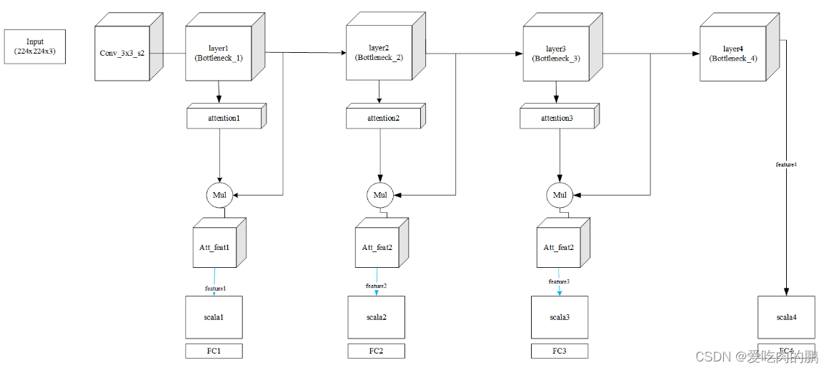
class ResNet(nn.Module):def __init__(self, block, layers, num_classes=100, zero_init_residual=False,groups=1, width_per_group=64, replace_stride_with_dilation=None,norm_layer=None):super(ResNet, self).__init__()if norm_layer is None:norm_layer = nn.BatchNorm2dself._norm_layer = norm_layerself.inplanes = 64# 空洞卷积定义self.dilation = 1# 是否用空洞卷积代替步长，如果不采用空洞卷积，均为Falseif replace_stride_with_dilation is None:# each element in the tuple indicates if we should replace# the 2x2 stride with a dilated convolution insteadreplace_stride_with_dilation = [False, False, False]if len(replace_stride_with_dilation) != 3:raise ValueError("replace_stride_with_dilation should be None ""or a 3-element tuple, got {}".format(replace_stride_with_dilation))self.groups = groups  # 分组卷积分组数self.base_width = width_per_group  # 卷积宽度# conv1与原始Resnet不同，原始Resnet为7x7卷积self.conv1 = nn.Conv2d(3, self.inplanes, kernel_size=3, stride=1, padding=1,bias=False)# bn层self.bn1 = norm_layer(self.inplanes)# relu激活函数self.relu = nn.ReLU(inplace=True)# 最大池化，不过在forward中没有用到self.maxpool = nn.MaxPool2d(kernel_size=3, stride=2, padding=1)self.layer1 = self._make_layer(block, 64, layers[0])  # 尺寸不变self.layer2 = self._make_layer(block, 128, layers[1], stride=2,dilate=replace_stride_with_dilation[0])  # 尺寸减半self.layer3 = self._make_layer(block, 256, layers[2], stride=2,dilate=replace_stride_with_dilation[1])  # 尺寸减半self.layer4 = self._make_layer(block, 512, layers[3], stride=2,dilate=replace_stride_with_dilation[2])  # 尺寸减半'''此处和原Resnet不同，原Resnet这里是自适应平均池化，然后接一个全连接层。scala层的作用是对特征层的H，W做缩放处理，因为要和深层网络中其他Bottleneck输出特征层之间做loss'''self.scala1 = nn.Sequential(# 输入通道64*4=256，输出通道128*4=512SepConv(  # 尺寸减半channel_in=64 * block.expansion,channel_out=128 * block.expansion),# 输入通道128*4=512， 输出通道256*4=1024SepConv(  # 尺寸减半channel_in=128 * block.expansion,channel_out=256 * block.expansion),# 输入通道256*4=1024，输出通道512*4=2048SepConv(  # 尺寸减半channel_in=256 * block.expansion,channel_out=512 * block.expansion),# 平均池化nn.AvgPool2d(4, 4))self.scala2 = nn.Sequential(# 输入通道128*4=512，输出通道1024SepConv(channel_in=128 * block.expansion,channel_out=256 * block.expansion,),# 输入通道256*4=1024，输出通道512*4=2048SepConv(channel_in=256 * block.expansion,channel_out=512 * block.expansion,),# 平均池化nn.AvgPool2d(4, 4))self.scala3 = nn.Sequential(# 输入通道256*4=1024，输出通道512*4=2048SepConv(channel_in=256 * block.expansion,channel_out=512 * block.expansion,),# 平均池化nn.AvgPool2d(4, 4))# 平均池化self.scala4 = nn.AvgPool2d(4, 4)self.attention1 = nn.Sequential(SepConv(  # 尺寸减半channel_in=64 * block.expansion,  # 256channel_out=64 * block.expansion  # 256),  # 比输入前大两个像素nn.BatchNorm2d(64 * block.expansion),nn.ReLU(),nn.Upsample(scale_factor=2, mode='bilinear'),  # 恢复原来尺寸nn.Sigmoid())self.attention2 = nn.Sequential(SepConv(channel_in=128 * block.expansion,channel_out=128 * block.expansion),nn.BatchNorm2d(128 * block.expansion),nn.ReLU(),nn.Upsample(scale_factor=2, mode='bilinear'),nn.Sigmoid())self.attention3 = nn.Sequential(SepConv(channel_in=256 * block.expansion,channel_out=256 * block.expansion),nn.BatchNorm2d(256 * block.expansion),nn.ReLU(),nn.Upsample(scale_factor=2, mode='bilinear'),nn.Sigmoid())self.fc1 = nn.Linear(512 * block.expansion, num_classes)self.fc2 = nn.Linear(512 * block.expansion, num_classes)self.fc3 = nn.Linear(512 * block.expansion, num_classes)self.fc4 = nn.Linear(512 * block.expansion, num_classes)for m in self.modules():if isinstance(m, nn.Conv2d):nn.init.kaiming_normal_(m.weight, mode='fan_out', nonlinearity='relu')elif isinstance(m, (nn.BatchNorm2d, nn.GroupNorm)):nn.init.constant_(m.weight, 1)nn.init.constant_(m.bias, 0)# Zero-initialize the last BN in each residual branch,# so that the residual branch starts with zeros, and each residual block behaves like an identity.# This improves the model by 0.2~0.3% according to https://arxiv.org/abs/1706.02677if zero_init_residual:for m in self.modules():if isinstance(m, Bottleneck):nn.init.constant_(m.bn3.weight, 0)elif isinstance(m, BasicBlock):nn.init.constant_(m.bn2.weight, 0)def _make_layer(self, block, planes, blocks, stride=1, dilate=False):norm_layer = self._norm_layerdownsample = Noneprevious_dilation = self.dilationif dilate:self.dilation *= stridestride = 1# 残差边采用1x1卷积升维条件，即当步长不为1或者输入通道数不等于输出通道数的时候if stride != 1 or self.inplanes != planes * block.expansion:downsample = nn.Sequential(conv1x1(self.inplanes, planes * block.expansion, stride),norm_layer(planes * block.expansion),)# layers用来存储每个当前残差层的所有残差块layers = []layers.append(block(self.inplanes, planes, stride, downsample, self.groups,self.base_width, previous_dilation, norm_layer))self.inplanes = planes * block.expansionfor _ in range(1, blocks):layers.append(block(self.inplanes, planes, groups=self.groups,base_width=self.base_width, dilation=self.dilation,norm_layer=norm_layer))# 仅在第一个bottleneck采用1x1进行升维，其他的bottleneck是直接输入和输出相加return nn.Sequential(*layers)def forward(self, x):# 以x = (1,3,224,224)为例feature_list = []x = self.conv1(x)  # get 1,64,224,224x = self.bn1(x)x = self.relu(x)x = self.layer1(x)  # conv2_x  输出256通道  1,256,224,224fea1 = self.attention1(x)  # 输出通道为256 224,224fea1 = fea1 * xfeature_list.append(fea1)x = self.layer2(x)  # conv3_x  1,512,112,112fea2 = self.attention2(x)  # 512,112,112fea2 = fea2 * xfeature_list.append(fea2)x = self.layer3(x)  # conv4_x 1,1024,56,56fea3 = self.attention3(x)  # 1024,56,56fea3 = fea3 * xfeature_list.append(fea3)x = self.layer4(x)  # conv5_x  最深层网络 1,2048,28,28feature_list.append(x)# feature_list[0].shape is [1,256 224,224] scala1 shape is [1,2048,7,7] view is [1,7*7*2048]out1_feature = self.scala1(feature_list[0]).view(x.size(0), -1)  # # 得到新的特征图 对应到论文中的Bottleneck1# feature_list[1].shape is [1,512,112,112], scala2 shape is [1,2048,7,7] view is [1,7*7*2048]out2_feature = self.scala2(feature_list[1]).view(x.size(0), -1)  # 得到新的特征图 对应到论文中的Bottleneck2# feature_list[2].shape is [1,1024,56,56],scala3 shape is [1,2048,7,7] view is [1,7*7*2048]out3_feature = self.scala3(feature_list[2]).view(x.size(0), -1)  # 得到新的特征图 对应到论文中的Bottleneck3# feature_list[3].shape is [1,2048,28,28],scala4 shape is [1,2048,7,7], view is [1,2048*7*7]out4_feature = self.scala4(feature_list[3]).view(x.size(0), -1)  # conv5_x  最深层网络out1 = self.fc1(out1_feature)out2 = self.fc2(out2_feature)out3 = self.fc3(out3_feature)out4 = self.fc4(out4_feature)# 返回的特征层分别是经过全连接和不仅过全连接的return [out4, out3, out2, out1], [out4_feature, out3_feature, out2_feature, out1_feature]

根据上述代码，网络结构图可以参考下面的。

可以这样描述，这里以输入大小为224x224x3为例，layer1就是残差块，除了第一个layer1不会改变特征层H和W，其他的layer输出后H和W均减半。同时在每个layer下会有个attention层（除了layer4），Att_feat是得到注意力后的特征图，然后通过scala均固定为大小[batch_szie,2048,7,7]，最后通过FC输出。

从代码来看，返回的有两个部分：1.经过FC层；2.没有经过FC层的输出

知识蒸馏训练

上面已经完成了网络的定义，下面看训练部分代码详解。

inputs是图像，labels是对应的标签。

net就是我们前面定义的Resnet网络。输出有两个部分(上面提到过)，outputs是经过FC，outputs_feature是没有经过FC的。前者是逻辑输出，后者是特征输出。

inputs, labels = data  # inputs是图片，labels是对应标签
inputs, labels = inputs.to(device), labels.to(device)
outputs, outputs_feature = net(inputs)  # 获得4个分类特征层，outputs是经过fc层的，outputs_feature是仅缩放后的特征层

这里的teacher为最深层网络，也就是结构图中的layer4 ，这里获取的teacher_feature_size是2048*7*7【以最初输入大小为224x224为例】

layer_list = []
teacher_feature_size = outputs_feature[0].size(1)

 下面的循环就为获得各个学生层，所以索引index是从1开始。这里的student_feature_size也是2048*7*7。

for index in range(1, len(outputs_feature)):student_feature_size = outputs_feature[index].size(1)  # 取浅层的三个特征层(没有经过FC)layer_list.append(nn.Linear(student_feature_size, teacher_feature_size))

这里的outputs是经过FC的分类输出，outputs[0]是layer4的。损失函数为交叉熵。 

#   for deepest classifier   hard loss
loss += criterion(outputs[0], labels)

teacher_output是最深层的Layer4[经过FC层]，要用这个做逻辑蒸馏，teacher_feature是最深层的layer4[没有经过FC] ，要用这个做特征蒸馏。

teacher_output = outputs[0].detach()  # 取出最深层特征层
teacher_feature = outputs_feature[0].detach()  # 取出最深层特征层(没有经过FC)

遍历浅层的逻辑输出outputs。

1.将layer4[teacher的逻辑输出]和每个student的逻辑输出做损失函数，为逻辑蒸馏损失，soft loss。

2.将 student和labels的损失作为hard loss。

3.度量每个student和teacher之间的特征距离，为特征蒸馏，soft loss。

通过上述方法，就有了三个部分的损失，逻辑损失+学生自己的hard loss + 特征蒸馏损失。

            #   for shallow classifiersfor index in range(1, len(outputs)):#   logits distillation 对分类输出最soft_loss# 逻辑蒸馏，将教师网络的输出和每个浅层学生网络之间做逻辑蒸馏,Loss source2loss += CrossEntropy(outputs[index], teacher_output) * args.loss_coefficient  # KL_loss soft loss# loss source1loss += criterion(outputs[index], labels) * (1 - args.loss_coefficient)  # hard loss 学生自己的#   feature distillation  hint蒸馏# 特征蒸馏,loss source3if index != 1:loss += torch.dist(net.adaptation_layers[index-1](outputs_feature[index]), teacher_feature) * \\args.feature_loss_coefficient#   the feature distillation loss will not be applied to the shallowest classifier

代码为： 

if __name__ == "__main__":# 记录最高准确率best_acc = 0# 开始训练for epoch in range(args.epoch):# [0,0,0,0,0]correct = [0 for _ in range(5)]# [0,0,0,0,0]predicted = [0 for _ in range(5)]# 学习率衰减if epoch in [args.epoch // 3, args.epoch * 2 // 3, args.epoch - 10]:for param_group in optimizer.param_groups:param_group['lr'] /= 10# trainnet.train()sum_loss, total = 0.0, 0.0# 数据集的加载for i, data in enumerate(trainloader, 0):length = len(trainloader)  # 获取数据集长度inputs, labels = data  # inputs是图片，labels是对应标签inputs, labels = inputs.to(device), labels.to(device)outputs, outputs_feature = net(inputs)  # 获得4个分类特征层，outputs是经过fc层的，outputs_feature是仅缩放后的特征层ensemble = sum(outputs[:-1])/len(outputs)  # outputs[:-1]取出out4, out3, out2(即不包含最深层)ensemble.detach_()if init is False:  # hint层#   init the adaptation layers.#   we add feature adaptation layers here to soften the influence from feature distillation loss#   the feature distillation in our conference version :  | f1-f2 | ^ 2#   the feature distillation in the final version : |Fully Connected Layer(f1) - f2 | ^ 2layer_list = []teacher_feature_size = outputs_feature[0].size(1)  # outputs_feature[0]是最深层的预测特征层 outputs_feature[1:]是浅层网络(学生)的特征层for index in range(1, len(outputs_feature)):student_feature_size = outputs_feature[index].size(1)  # 取浅层的三个特征层(没有经过FC)layer_list.append(nn.Linear(student_feature_size, teacher_feature_size))net.adaptation_layers = nn.ModuleList(layer_list)net.adaptation_layers.cuda()optimizer = optim.SGD(net.parameters(), lr=args.init_lr, weight_decay=5e-4, momentum=0.9)#   define the optimizer here again so it will optimize the net.adaptation_layersinit = True#   compute lossloss = torch.FloatTensor([0.]).to(device)#   for deepest classifier   hard lossloss += criterion(outputs[0], labels)  # 最深层的特征层(经过FC输出)和labels计算交叉熵 [教师自己的]teacher_output = outputs[0].detach()  # 取出最深层特征层teacher_feature = outputs_feature[0].detach()  # 取出最深层特征层(没有经过FC)#   for shallow classifiersfor index in range(1, len(outputs)):#   logits distillation 对分类输出最soft_loss# 逻辑蒸馏，将教师网络的输出和每个浅层学生网络之间做逻辑蒸馏,Loss source2loss += CrossEntropy(outputs[index], teacher_output) * args.loss_coefficient  # KL_loss soft loss# loss source1loss += criterion(outputs[index], labels) * (1 - args.loss_coefficient)  # hard loss 学生自己的#   feature distillation  hint蒸馏# 特征蒸馏,loss source3if index != 1:loss += torch.dist(net.adaptation_layers[index-1](outputs_feature[index]), teacher_feature) * \\args.feature_loss_coefficient#   the feature distillation loss will not be applied to the shallowest classifiersum_loss += loss.item()optimizer.zero_grad()loss.backward()optimizer.step()total += float(labels.size(0))outputs.append(ensemble)for classifier_index in range(len(outputs)):_, predicted[classifier_index] = torch.max(outputs[classifier_index].data, 1)correct[classifier_index] += float(predicted[classifier_index].eq(labels.data).cpu().sum())print('[epoch:%d, iter:%d] Loss: %.03f | Acc: 4/4: %.2f%% 3/4: %.2f%% 2/4: %.2f%%  1/4: %.2f%%'' Ensemble: %.2f%%' % (epoch + 1, (i + 1 + epoch * length), sum_loss / (i + 1),100 * correct[0] / total, 100 * correct[1] / total,100 * correct[2] / total, 100 * correct[3] / total,100 * correct[4] / total))print("Waiting Test!")with torch.no_grad():correct = [0 for _ in range(5)]predicted = [0 for _ in range(5)]total = 0.0for data in testloader:net.eval()images, labels = dataimages, labels = images.to(device), labels.to(device)outputs, outputs_feature = net(images)ensemble = sum(outputs) / len(outputs)outputs.append(ensemble)for classifier_index in range(len(outputs)):_, predicted[classifier_index] = torch.max(outputs[classifier_index].data, 1)correct[classifier_index] += float(predicted[classifier_index].eq(labels.data).cpu().sum())total += float(labels.size(0))print('Test Set AccuracyAcc: 4/4: %.4f%% 3/4: %.4f%% 2/4: %.4f%%  1/4: %.4f%%'' Ensemble: %.4f%%' % (100 * correct[0] / total, 100 * correct[1] / total,100 * correct[2] / total, 100 * correct[3] / total,100 * correct[4] / total))if correct[4] / total > best_acc:best_acc = correct[4]/totalprint("Best Accuracy Updated: ", best_acc * 100)torch.save(net.state_dict(), "./checkpoints/"+str(args.model)+".pth")print("Training Finished, TotalEPOCH=%d, Best Accuracy=%.3f" % (args.epoch, best_acc))