Scillus | 来吧！它可以大大简化你的Seurat分析流程哦！~（二）（高级可视化）

1写在前面

不知道大家那里天气热了没有，苦逼的我虽然“享受”着医院的恒温，但也并没有什么卵用，毕竟我只是个不可以生锈的“小螺丝”。🥲

上期介绍了Scillus包的基本功能，如何进行数据的预处理及其可视化。🤨

本期我们继续吧，介绍其主要的一些高级功能吧，包括降维，统计，热图和富集分析等等。🤩

2用到的包

rm(list = ls())
library(tidyverse)
library(Scillus)
library(Seurat)
library(magrittr)
library(purrr)

3示例数据

我们用一下上次经过标准化处理后的scRNA_int，具体的可以回顾上一篇教程：👇

📍🧐 Scillus | 来吧！它可以大大简化你的Seurat分析流程哦！~（一）（数据预处理）

load("./scRNA_scillus.Rdata")

scRNA_int

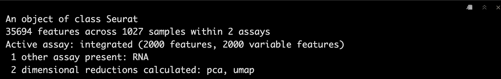
4降维及其可视化

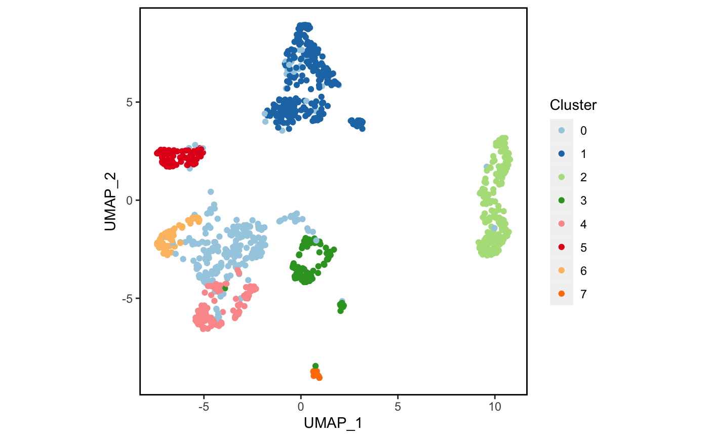
4.1 初步绘图

先来简单画一下吧。🥳

plot_scdata(scRNA_int, pal_setup = pal)

4.2 换个主题配色

换个配色试试。🥰

plot_scdata(scRNA_int, pal_setup = "Dark2")

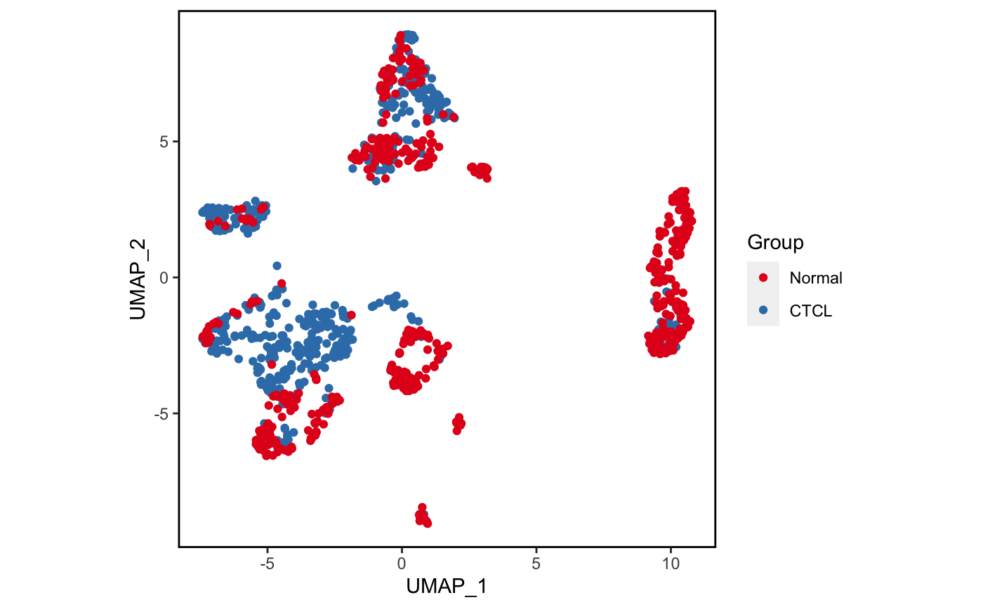
4.3 分组可视化

我们试试分组降维吧。🤒

plot_scdata(scRNA_int, color_by = "group", pal_setup = pal)

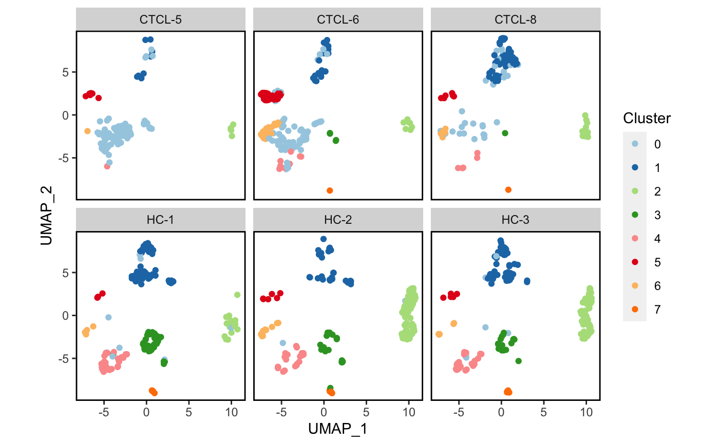
4.4 分面可视化

我们试一下按sample分面降维吧。🤒

plot_scdata(scRNA_int, split_by = "sample", pal_setup = pal)

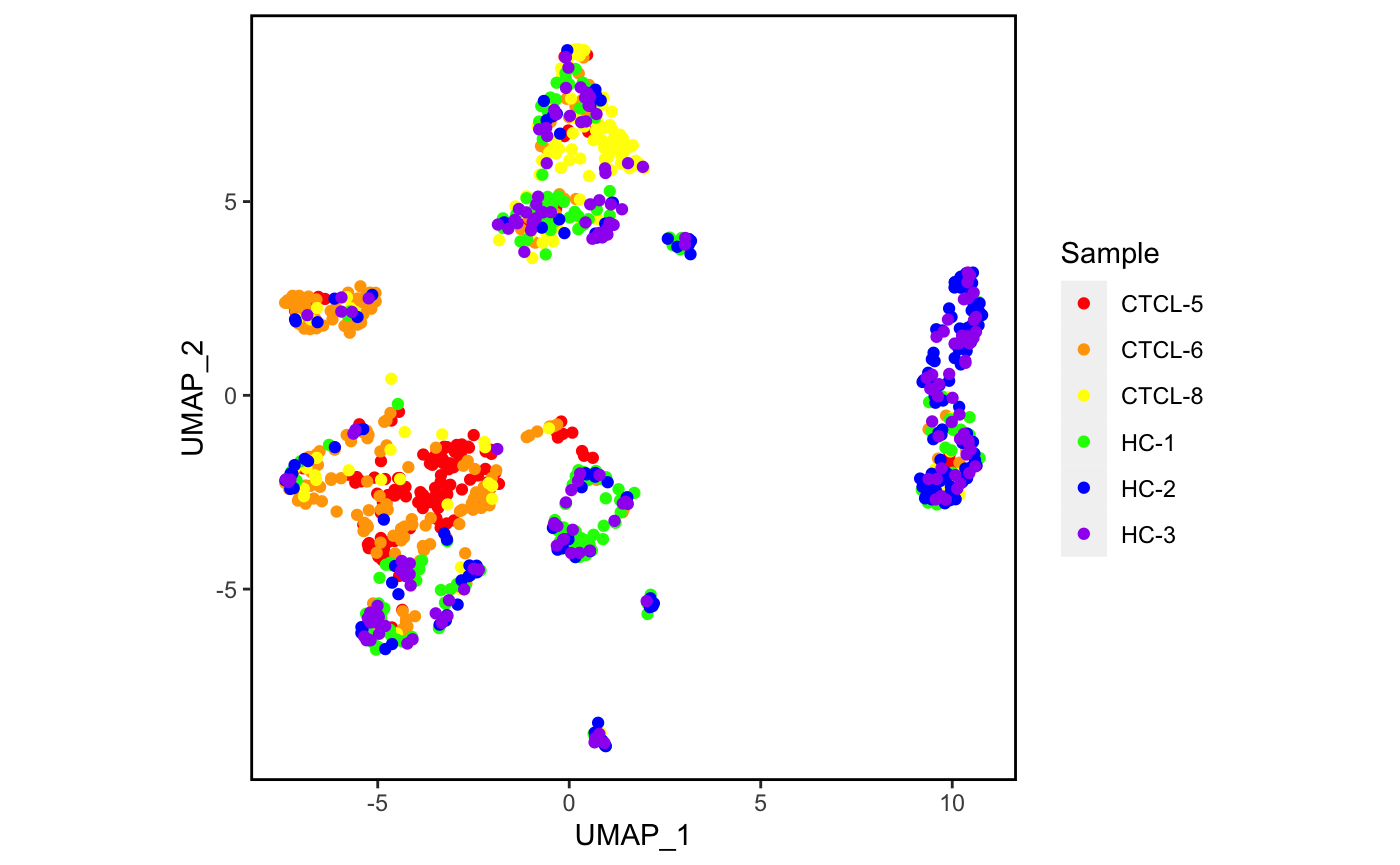
4.5 手动配色

我们再试着手动配色一下吧。🧐

plot_scdata(scRNA_int, color_by = "sample", 
            pal_setup = c("red","orange","yellow","green","blue","purple"))

5统计及其可视化

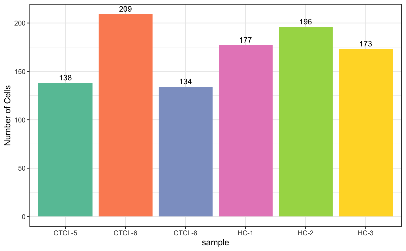
5.1 按sample统计

plot_stat(scRNA_int, 
          plot_type = "group_count"
          ## 三种，"group_count", "prop_fill", and "prop_multi"
          )

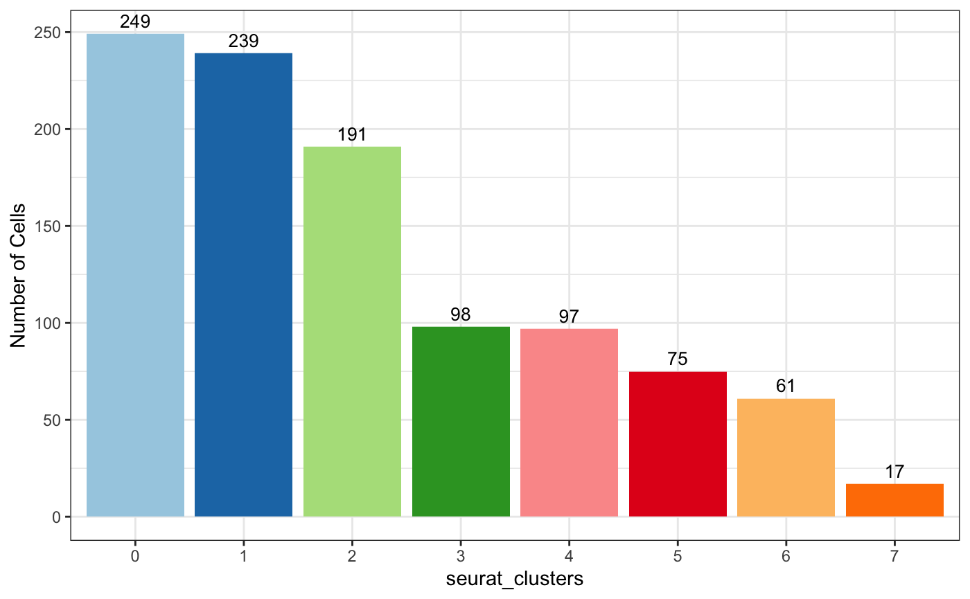
5.2 按cluster统计

plot_stat(scRNA_int, "group_count", group_by = "seurat_clusters", pal_setup = pal)

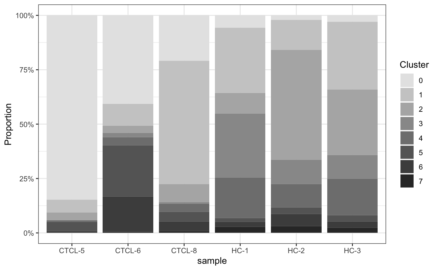
5.3 堆叠柱形图

plot_stat(scRNA_int, 
          plot_type = "prop_fill", 
          pal_setup = c("grey90","grey80","grey70","grey60","grey50","grey40","grey30","grey20"))

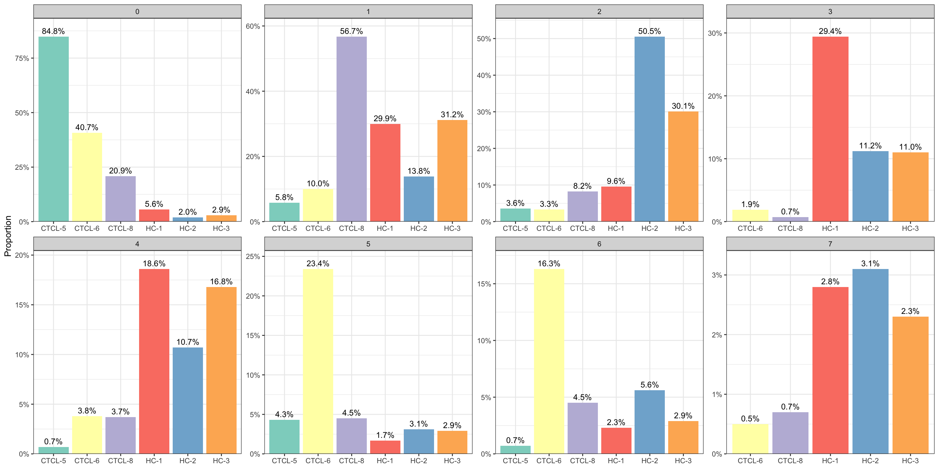
5.4 按cluster和sample统计

plot_stat(scRNA_int, plot_type = "prop_multi", pal_setup = "Set3")

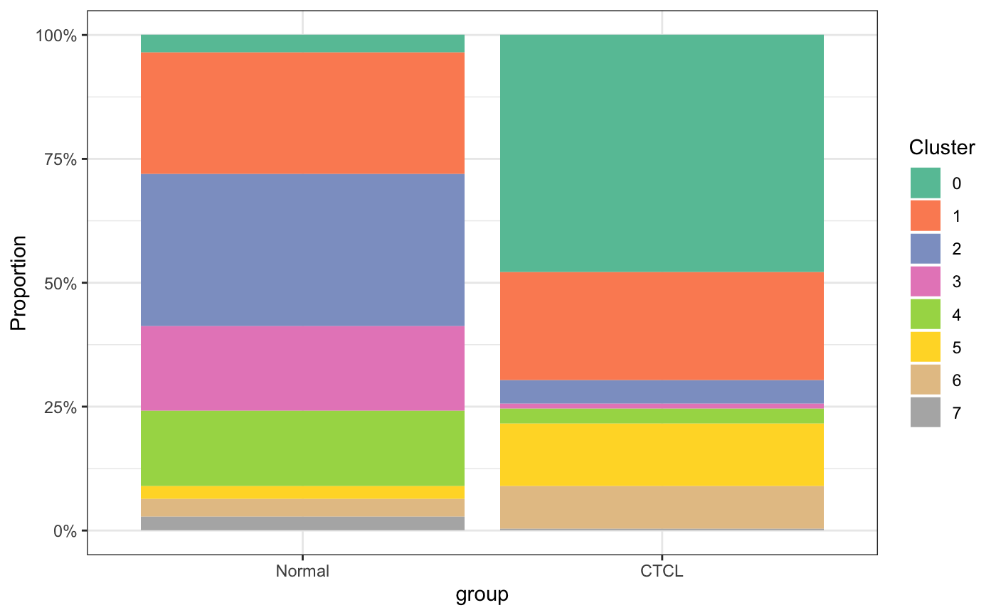
5.5 按cluster和group统计

plot_stat(scRNA_int, plot_type = "prop_fill", group_by = "group")

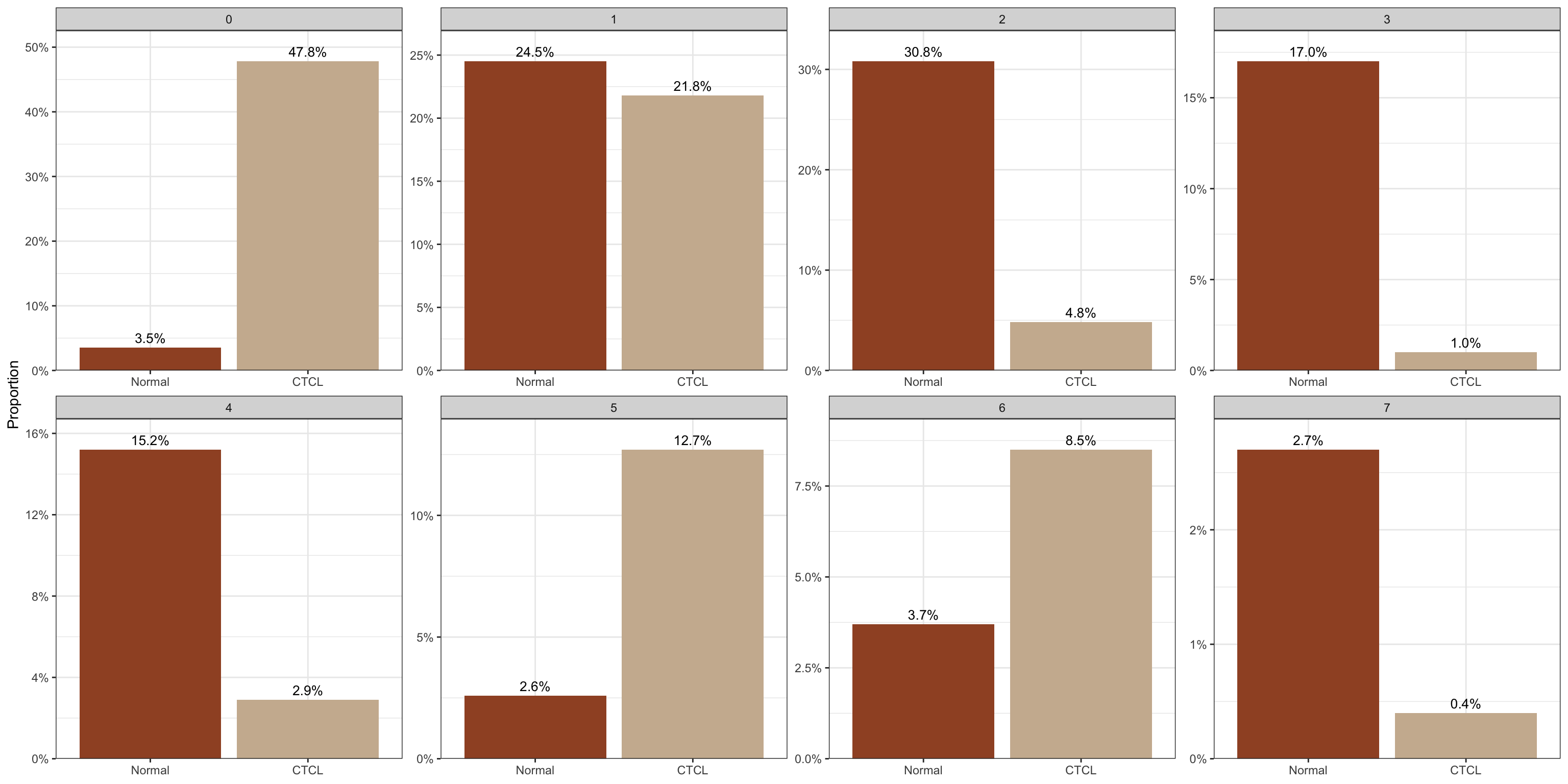
5.6 换个配色

plot_stat(scRNA_int, plot_type = "prop_multi", 
          group_by = "group", pal_setup = c("sienna","bisque3"))

6热图及其可视化

6.1 寻找marker

我们首先要用Seurat包的FindAllMarkers确定一下marker，分析方法也比较多，包括wilcox, roc, t, poisson, DESeq2等。😷

markers <- FindAllMarkers(scRNA_int, logfc.threshold = 0.25, min.pct = 0.1, only.pos = F)

6.2 热图可视化

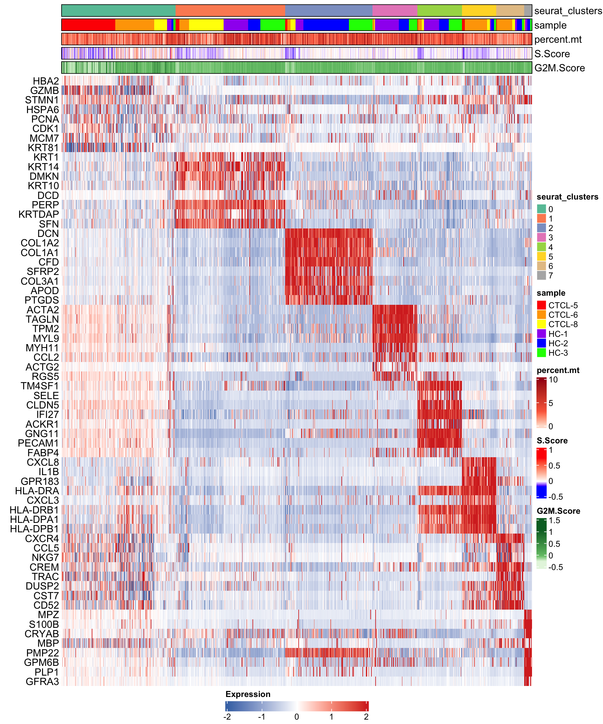
在热图中，每一行代表一个基因，每一列代表一种细胞，默认绘制每种细胞的前8个基因。🤓

细胞可以通过sort_var进行排序，默认设置为c("seurat_clusters")，即细胞按cluster进行排序。🙃

当然你也可以在sort_var中指定多个变量，然后按多个变量进行排序。🥳

anno_var用来指定注释数据或者metadata中的相关数据。🥰

plot_heatmap(dataset = scRNA_int, 
              markers = markers,
              sort_var = c("seurat_clusters","sample"),
              anno_var = c("seurat_clusters","sample","percent.mt","S.Score","G2M.Score"),
              anno_colors = list("Set2",                                             
                                 # RColorBrewer palette
                                 c("red","orange","yellow","purple","blue","green"), 
                                 # color vector
                                 "Reds",
                                 c("blue","white","red"),                            
                                 # Three-color gradient
                                 "Greens"))

6.3 调整热图

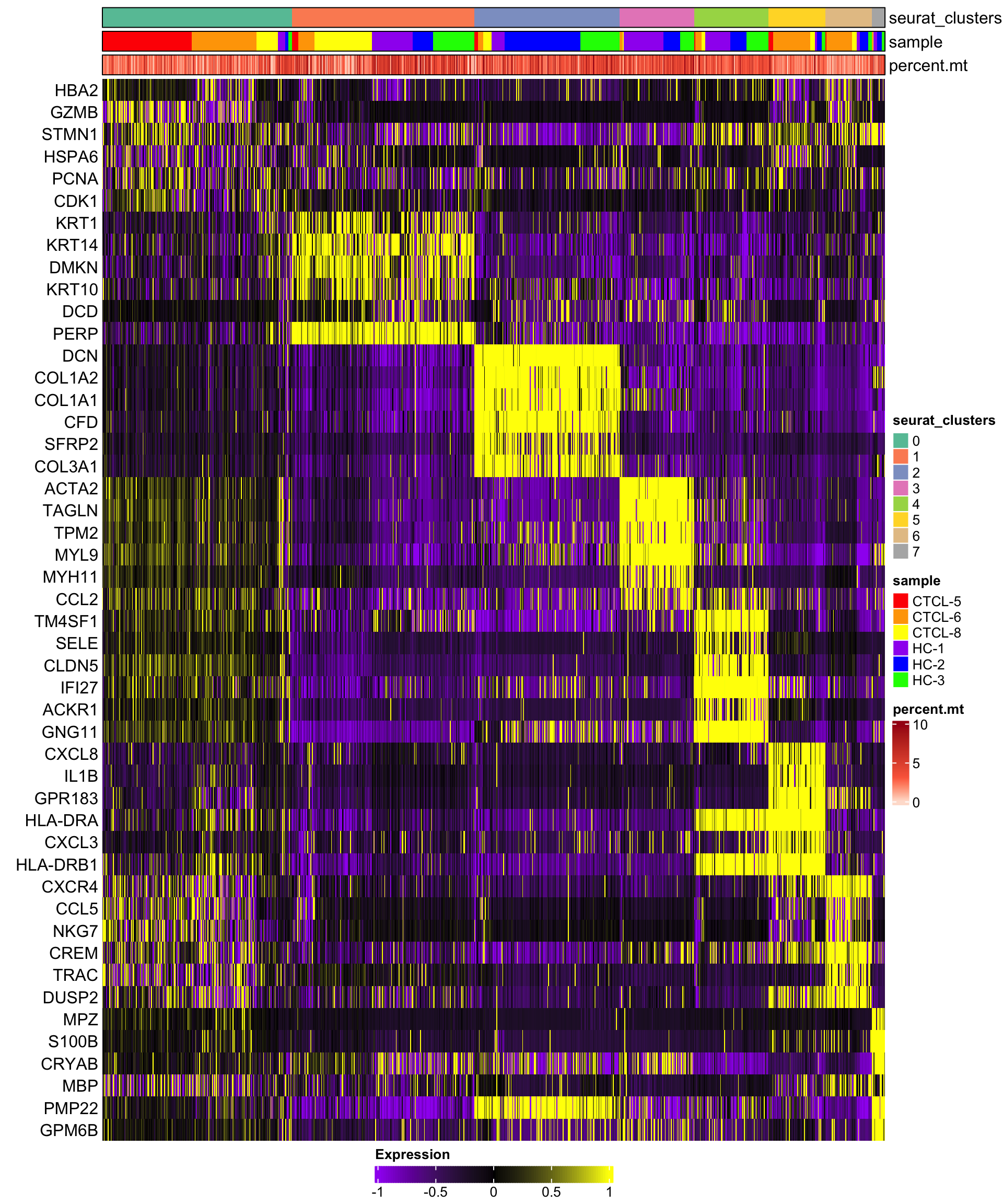
我们调一下limit和渐变的配色, 显示前6个基因。😂

plot_heatmap(dataset = scRNA_int,
             n = 6,
             markers = markers,
             sort_var = c("seurat_clusters","sample"),
             anno_var = c("seurat_clusters","sample","percent.mt"),
             anno_colors = list("Set2",
                                c("red","orange","yellow","purple","blue","green"),
                                "Reds"),
             hm_limit = c(-1,0,1),
             hm_colors = c("purple","black","yellow"))

7富集分析

7.1 制定cluster的GO分析

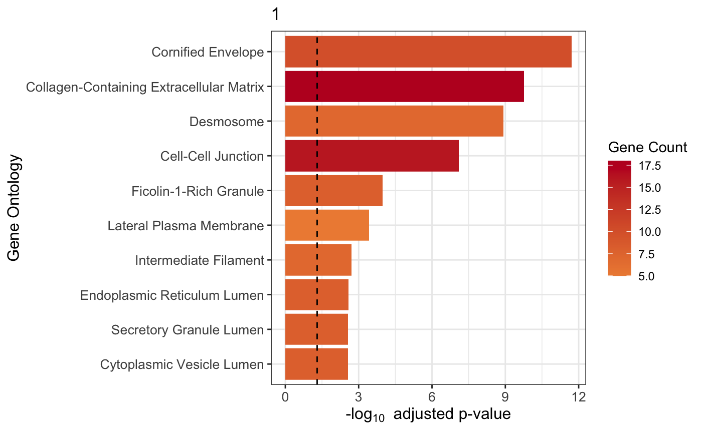
我们指定cluster 1的GO分析试试。🐵

plot_cluster_go(markers, cluster_name = "1", org = "human", ont = "CC")

7.2 所有cluster的GO分析

再试试绘制所有cluster的GO分析。🐵

plot_all_cluster_go(markers, org = "human", ont = "BP")

8GSEA分析

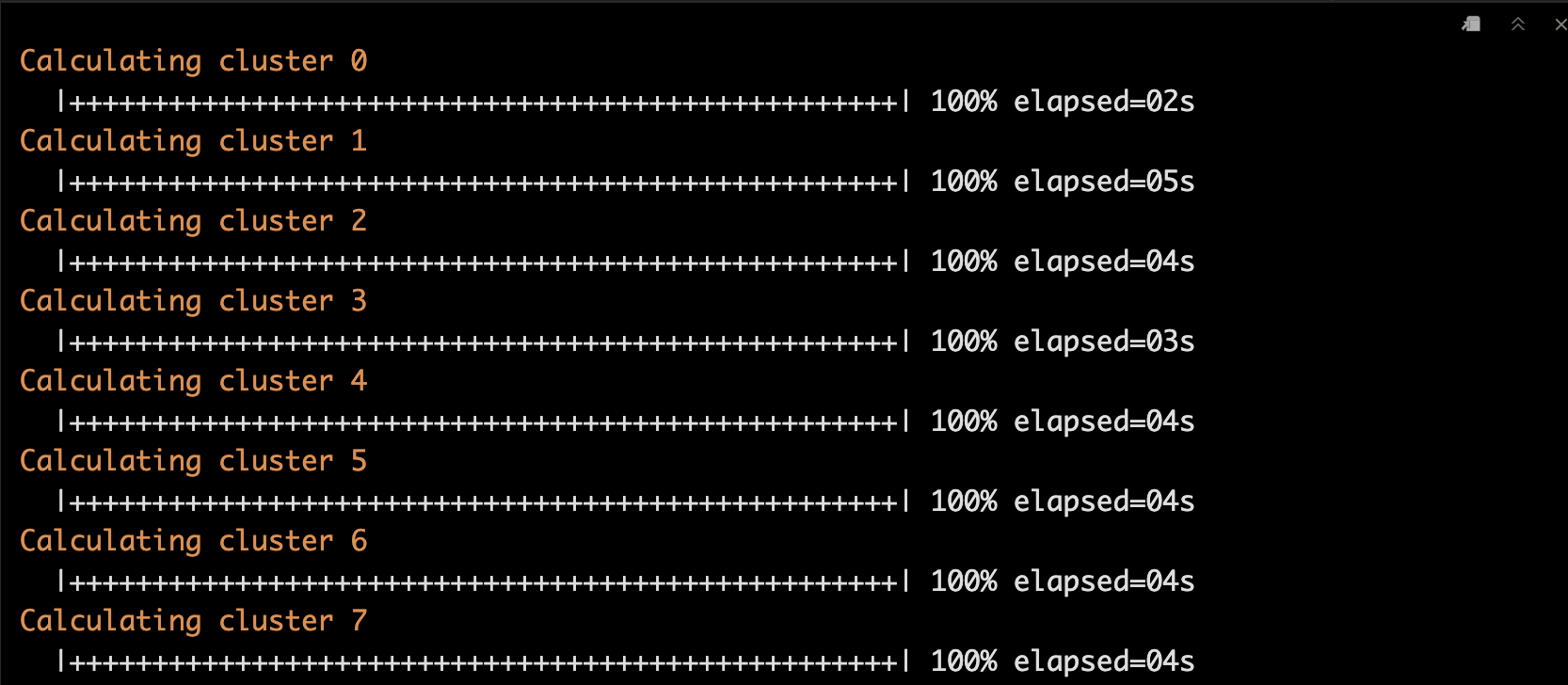
8.1 差异分析

首先我们要用find_diff_genes做一下差异分析，寻找差异基因。😜

然后使用test_GSEA()进行GSEA分析。

de <- find_diff_genes(dataset = scRNA_int, 
                      clusters = as.character(0:7),
                      comparison = c("group", "CTCL", "Normal"),
                      logfc.threshold = 0,   # threshold of 0 is used for GSEA
                      min.cells.group = 1)   # To include clusters with only 1 cell

gsea_res <- test_GSEA(de, 
                      pathway = pathways.hallmark)

8.2 GSEA结果可视化

plot_GSEA(gsea_res, p_cutoff = 0.1, colors = c("#0570b0", "grey", "#d7301f"))

9补充一下

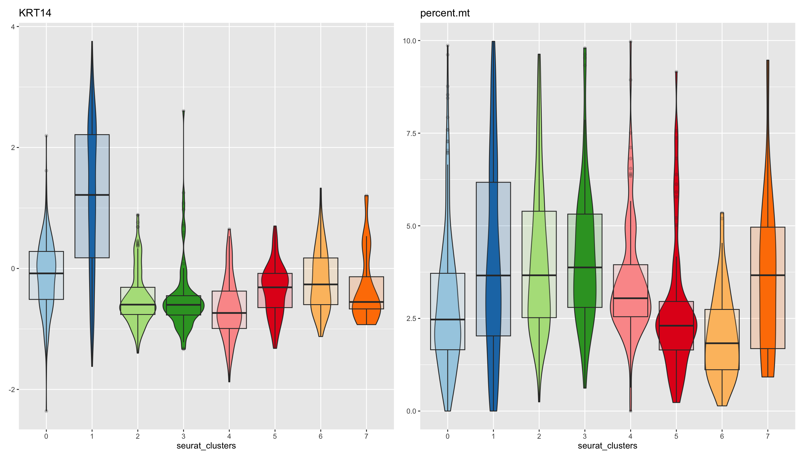
在Scillus包中有一个非常好用的功能叫Plotting Measures，在这里补充一下。😜

在设置的参数中measures = 你需要的基因或指标就可以啦。🧐

9.1 小试牛刀

plot_measure(dataset = scRNA_int, 
             measures = c("KRT14","percent.mt"), 
             group_by = "seurat_clusters", 
             pal_setup = pal)

9.2 更进一步

plot_measure_dim(dataset = scRNA_int, 
                 measures = c("nFeature_RNA","nCount_RNA","percent.mt","KRT14"),
                 split_by = "sample")

最后祝大家早日不卷!~

点个在看吧各位~ ✐.ɴɪᴄᴇ ᴅᴀʏ 〰

📍 往期精彩