经验正交分解EOF的Matlab的实现示例

文章列表

在地学中，PCA和EOF通常用于信号提取，从繁杂的时空数据中分离出地理要素的时空变化特征，是进行地学信号分析的前提。本质上PCA和EOF没有什么不同，只是：EOF为空间特征向量，也称为空间模态，在一定程度上反映了要素场的空间分布特点；PC（主成分）对应时间变化，也称为时间系数，反映相应空间模态（EOF）随时间的权重变化。简而言之，二者是利用经验正交分解过程中的两个重要元素。

下面我略过基本概念的介绍，直接给出一个Matlab进行EOF分解的示例代码：

1.加载数据

% Load sample data:
load pacific_sst.mat
% Calculate the first EOF of sea surface temperatures and its
% principal component time series:
[eofmap,pc] = eof(sst,1);
% Plot the first EOF map:
imagescn(lon,lat,eofmap);
axis xy image off
% Optional: Use a cmocean colormap:
cmocean('delta','pivot',0)

得到的是海温数据集的第一个EOF

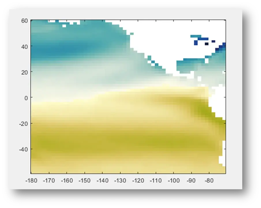
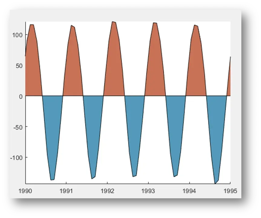
但由于我们没有去掉季节周期，第一个EOF主要代表季节变化。作为上述模式与季节周期相关的证据，看看相应的主成分时间序列。

figure
anomaly(t,pc)
axis tight
xlim([datenum('jan 1, 1990') datenum('jan 1, 1995')])
datetick('x','keeplimits')

2. 计算平均的海洋温度数据，并展示多年的平均温度

figure
imagescn(lon,lat,mean(sst,3));
axis xy off
cb = colorbar;
ylabel(cb,' mean temperature {\\circ}C ')
cmocean thermal

3. 计算1950年至2016年的线性变化趋势，请确保将趋势乘以10*365.25，以将每天的度数转换为每十年的度数:

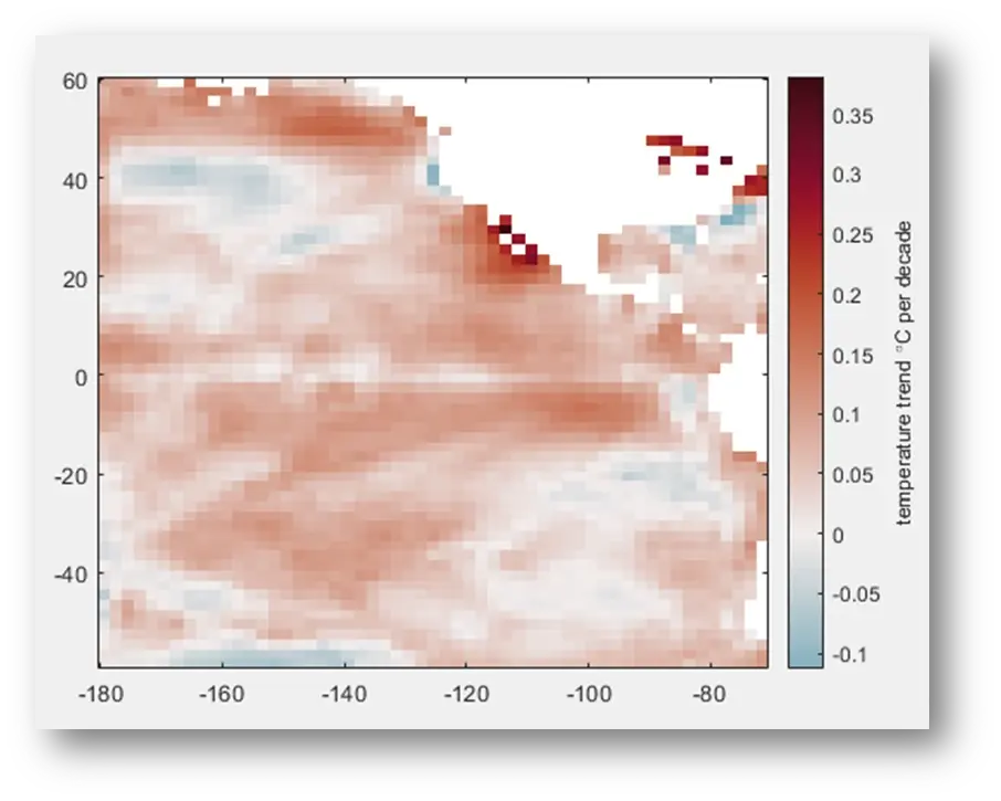
为了移除季节项和趋势项对异常信号的影响，我们接下来对数据进行去趋势和去周期处理

sst = detrend3(sst,t);
sst = deseason(sst,t);

所以现在我们的海温数据已经去趋势化了，均值被去除了，季节周期也被去除了。海温中剩下的都是异常现象——变化的东西，但不是长期趋势或短期年度周期。这是我们海温异常数据集的剩余方差:

4. 接着计算EOF前三个模态

figure
subsubplot(3,1,1)
plot(t,pc(1,:))
box off
axis tight
ylabel 'pc1'
title 'The first three principal components'subsubplot(3,1,2)
plot(t,pc(2,:))
box off
axis tight
set(gca,'yaxislocation','right')
ylabel 'pc2'subsubplot(3,1,3)
plot(t,pc(3,:))
box off
axis tight
ylabel 'pc3'
datetick('x','keeplimits')

5. El Niño南方涛动(ENSO)时间序列，果然，有记录以来最强的厄尔尼诺现象发生在1982-1983年、1997-1998年和2014-2016年。

figure('pos',[100 100 600 250])
anomaly(t,-pc(1,:),'topcolor',rgb('bubblegum'),...'bottomcolor',rgb('periwinkle blue')) % First principal component is enso
box off
axis tight
datetick('x','keeplimits')
text([724316 729713 736290],[.95 .99 .81],'El Nino','horiz','center')

有时我们听说厄尔尼诺现象的特征频率是每5年一次，或者5到7年一次，有时你听说是每2到7年一次。在时间序列中很难看到这一点，所以我们用plotpsd绘制频域的第一个主成分，指定每年12个样本的采样频率，绘制在log x轴上，x值以lambda(年)为单位，而不是频率:

figure
plotpsd(pc(1,:),12,'logx','lambda')
xlabel 'periodicity (years)'
set(gca,'xtick',[1:7 33])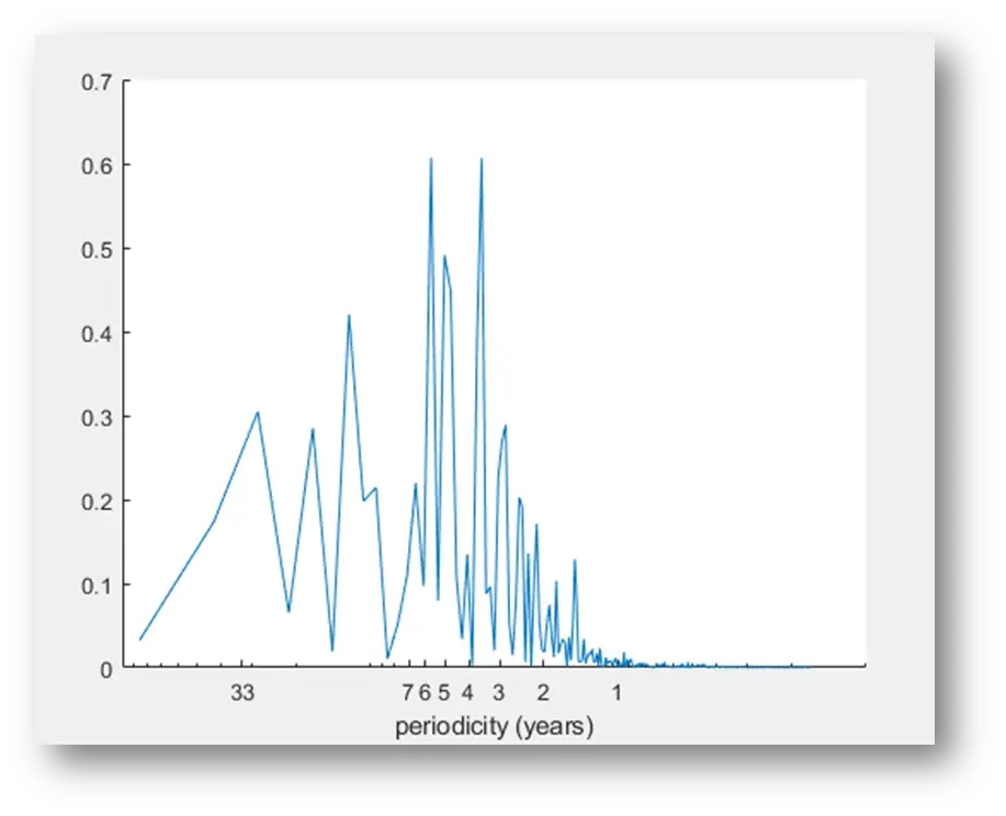

下面是前6个模态的空间分布：

s = [-1 1 -1 1 -1 1]; % (sign multiplier to match Messie and Chavez 2011)figure('pos',[100 100 500 700])
for k = 1:6subplot(3,2,k)imagescn(lon,lat,eof_maps(:,:,k)*s(k));axis xy offtitle(['Mode ',num2str(k),' (',num2str(expv(k),'%0.1f'),'%)'])caxis([-2 2])
endcolormap jet

在任何给定时间，通过绘制上图所示的模态1的图，乘以其对应的主成分(向量pc(1，:)))，都可以获得与ENSO相关的海面温度异常的快照。同样地，你可以通过将所有EOF图加起来，再乘以当时对应的主成分，得到给定时间内全球海面温度异常的图像。通过这种方式，我们可以建立一个越来越完整的海温异常电影，因为我们包括越来越多的变率模态。

例如，在特定时间内，与前三个变率模态相关的海温异常图可以通过将每个模态的eof图相加，乘以相应的pc值来获得。这样计算90年代的总和:

% Indices of start and end dates for the movie:
startind = find(t>=datenum('jan 1, 1990'),1,'first');
endind = find(t<=datenum('dec 31, 1999'),1,'last');
% A map of SST anomalies from first three modes at start:
map = eof_maps(:,:,1)*pc(1,startind) + ... % Mode 1, Jan 1990eof_maps(:,:,2)*pc(2,startind) + ... % Mode 2, Jan 1990eof_maps(:,:,3)*pc(3,startind);      % Mode 3, Jan 1990
sst_f = reof(eof_maps,pc,1:3);
ind_1990s = 481:3:600; % (every third value to cut down on gif size)
figure
h = imagescn(sst_f(:,:,ind_1990s(1)));
caxis([-2 2])
cmocean balance
cb = colorbar;
ylabel(cb,'temperature anomaly (modes 1-3)')
title(datestr(t(ind_1990s(1)),'yyyy'))
gif('SSTs_1990s.gif','frame',gcf) % writes the first frame
for k = 2:length(ind_1990s)h.CData = sst_f(:,:,ind_1990s(k));title(datestr(t(ind_1990s(k)),'yyyy'))gif % adds this frame to the gif
end

参考资料：

主成分分析PCA和经验正交函数分析EOF的原理（通俗易懂的解释）_a99h的博客-CSDN博客
Messié, Monique, and Francisco Chavez. "Global modes of sea surface temperature variability in relation to regional climate indices." Journal of Climate 24.16 (2011): 4314-4331. doi:10.1175/2011JCLI3941.1.
Rayner, N. A., Parker, D. E., Horton, E. B., Folland, C. K., Alexander, L. V., Rowell, D. P., Kent, E. C., Kaplan, A. (2003). Global analyses of sea surface temperature, sea ice, and night marine air temperature since the late nineteenth century. J. Geophys. Res.Vol. 108, No. D14, 4407 doi:10.1029/2002JD002670.
Thyng, K.M., C.A. Greene, R.D. Hetland, H.M. Zimmerle, and S.F. DiMarco. 2016. True colors of oceanography: Guidelines for effective and accurate colormap selection. Oceanography 29(3):9-13, doi:10.5670/oceanog.2016.66.

Matlab程序和数据下载：

链接：https://pan.baidu.com/s/1IrlhONl8V9ubuykuy7yq_g?pwd=ucas提取码：ucas

欢迎点赞收藏！

经验正交分解EOF的Matlab的实现示例

相关问题

公告