机器学习入门实例-加州房价预测-1(数据准备与可视化)

问题描述
数据来源:California Housing Prices dataset from the StatLib repository,1990年加州的统计数据。
要求:预测任意一个街区的房价中位数
缩小问题:superwised multiple regressiong(用到人口、收入等特征) univariate regression(只预测一个数据)plain batch learning(数据量不大+不咋变动)
准备数据
下载数据
可以去github,也可以自动下载。
import os
import tarfile
import urllib.request
import pandas as pddown_root = "https://raw.githubusercontent.com/ageron/handson-ml2/master/"
HOUSING_PATH = "datasets"
HOUSING_URL = down_root + "datasets/housing/housing.tgz"def fetch_housing_data(housing_url=HOUSING_URL, housing_path=HOUSING_PATH):tgz_path = os.path.join(housing_path, "housing.tgz")urllib.request.urlretrieve(housing_url, tgz_path)housing_tgz = tarfile.open(tgz_path)housing_tgz.extractall(path=housing_path)housing_tgz.close()
查看数据
def load_housing_data(housing_path=HOUSING_PATH):csv_path = os.path.join(housing_path, "housing.csv")return pd.read_csv(csv_path)housing = load_housing_data()
# housing.head() 默认打印前5行信息,中间列可能省略
# housing.info() 打印行列信息、类型等
housing.info()可以简单查看数据情况。可以看到,total_bedrooms里有数据缺失,而ocean_proximity的类型是object。因为文件是csv格式,所以肯定是字符串类型。
<class 'pandas.core.frame.DataFrame'>
RangeIndex: 20640 entries, 0 to 20639
Data columns (total 10 columns):#   Column              Non-Null Count  Dtype
---  ------              --------------  -----  0   longitude           20640 non-null  float641   latitude            20640 non-null  float642   housing_median_age  20640 non-null  float643   total_rooms         20640 non-null  float644   total_bedrooms      20433 non-null  float645   population          20640 non-null  float646   households          20640 non-null  float647   median_income       20640 non-null  float648   median_house_value  20640 non-null  float649   ocean_proximity     20640 non-null  object
dtypes: float64(9), object(1)
memory usage: 1.6+ MB
None
打印一下ocean_proximity的分类及统计,可以看到是标签,category
print(housing["ocean_proximity"].value_counts())<1H OCEAN     9136
INLAND        6551
NEAR OCEAN    2658
NEAR BAY      2290
ISLAND           5
Name: ocean_proximity, dtype: int64
housing.describe()可以计算各个数值列的count,mean,std,min,25%、50%和75%(中位数)、max。计算时null会被忽略。
也可以通过绘制柱形图观察数据。
import matplotlib.pyplot as plt
housing.hist(bins=50, figsize=(20,15))
plt.show()
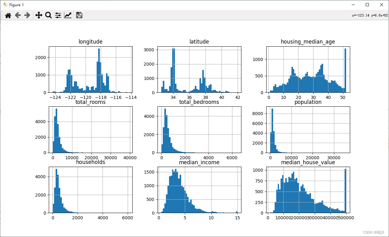
要看柱形图是因为某些机器学习算法更适合用正态数据,如果是tail-heavy(左偏)需要通过一些方法修正。
划分测试集与训练集
最简单的是直接随机挑选。但是要设置seed,因为如果不设置的话,每次运行得到的训练集不一样,时间长了整个训练集都是已知了,那测试集就失去意义了。
import numpy as np
def get_train_set(data, ratio=0.2):# 可以先设置seed以保持shuffled不变np.random.seed(42)shuffled = np.random.permutation(len(data))test_set_size = int(len(data) * ratio)test_indices = shuffled[:test_set_size]train_indices = shuffled[test_set_size:]return data.iloc[train_indices], data.iloc[test_indices]
同时scikit learn也提供了方法:random_state就跟前面设seed的功能一样。
from sklearn.model_selection import train_test_split
# random_state是随机种子,如果两次设置相同,则划分结果相同
train_set, test_set = train_test_split(housing, test_size=0.2, random_state=42)
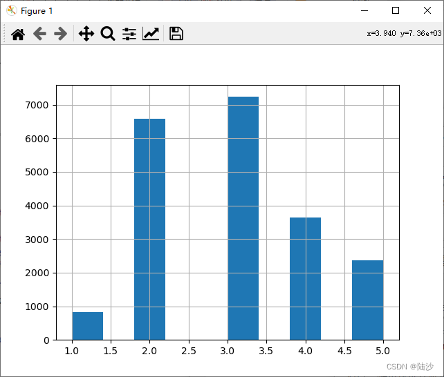
但是,随机挑选的数据可以不够有代表性。假设median income是一个重要的特性,需要对它进行分层抽样。先看一下数据分布:
housing["income_cat"] = pd.cut(housing["median_income"], bins=[0., 1.5, 3.0, 4.5, 6., np.inf],labels=[1,2,3,4,5])
housing["income_cat"].hist()
plt.show()
使用scikit learn带的分层抽样函数进行分层:
from sklearn.model_selection import StratifiedShuffleSplit# n_splits 参数指定了要生成的划分数量. 1就是生成1种随机划分
split = StratifiedShuffleSplit(n_splits=1, test_size=0.2, random_state=42)
for train_index, test_index in split.split(housing, housing["income_cat"]):strat_train_set = housing.loc[train_index]strat_test_set = housing.loc[test_index]
print(strat_test_set)
此时可以看到,
       longitude  latitude  ...  ocean_proximity  income_cat
5241     -118.39     34.12  ...        <1H OCEAN           5
17352    -120.42     34.89  ...        <1H OCEAN           4
3505     -118.45     34.25  ...        <1H OCEAN           3
7777     -118.10     33.91  ...        <1H OCEAN           3
14155    -117.07     32.77  ...       NEAR OCEAN           3
...          ...       ...  ...              ...         ...
12182    -117.29     33.72  ...        <1H OCEAN           2
7275     -118.24     33.99  ...        <1H OCEAN           2
17223    -119.72     34.44  ...        <1H OCEAN           4
10786    -117.91     33.63  ...        <1H OCEAN           4
3965     -118.56     34.19  ...        <1H OCEAN           3[4128 rows x 11 columns]
验证一下是否正确分层抽样了:
print(strat_test_set["income_cat"].value_counts() / len(strat_test_set))3    0.350533
2    0.318798
4    0.176357
5    0.114341
1    0.039971
Name: income_cat, dtype: float64
最终函数为:
def get_train_test_split(data, test_size):# 完全随机分类# from sklearn.model_selection import train_test_split# random_state是随机种子,如果两次设置相同,则划分结果相同# test_size是测试集所占的比例 0-1# train_set, test_set = train_test_split(data, test_size=test_size, random_state=42)# return train_set, test_set# 需要对某一列进行分层抽样# 先创造一个新列,根据某列内容,给各行打上标签data["income_cat"] = pd.cut(housing["median_income"],bins=[0., 1.5, 3.0, 4.5, 6., np.inf],labels=[1, 2, 3, 4, 5])from sklearn.model_selection import StratifiedShuffleSplit# n_splits 参数指定了要生成的划分数量split = StratifiedShuffleSplit(n_splits=1, test_size=test_size, random_state=42)for train_index, test_index in split.split(data, data["income_cat"]):strat_train_set = data.loc[train_index]strat_test_set = data.loc[test_index]# 删除刚才创造的新列for set_ in (strat_train_set, strat_test_set):# axis=1表示删除列set_.drop("income_cat", axis=1, inplace=True)return strat_train_set, strat_test_set
数据可视化
train_set, test_set = get_train_test_split(housing, 0.2)visual_data = train_set.copy()# alpha=0是透明,1是实心visual_data.plot(kind="scatter", x="longitude", y="latitude", alpha=0.1)plt.show()
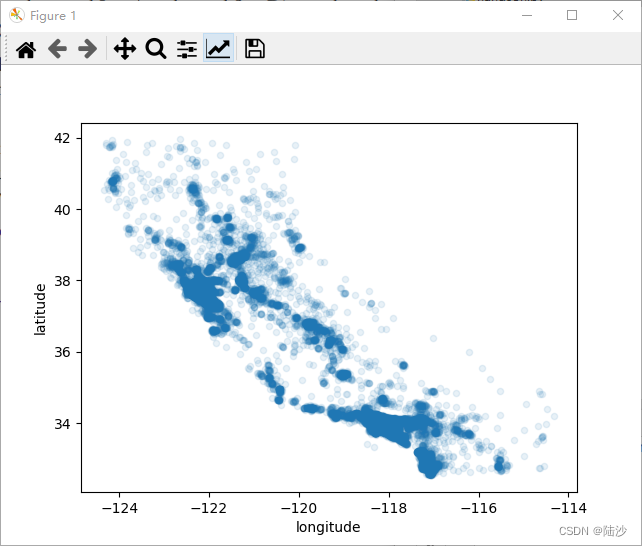
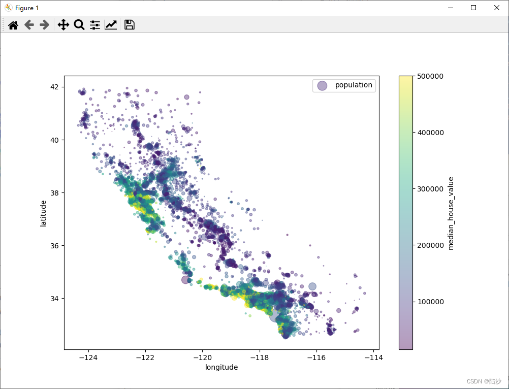
换一种包含信息更多的方式:令散点的直径大小表示人口,颜色表示房价中位值。
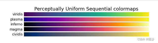
# s是指定散点图中点的大小,figsize默认(6.4, 4.8)格式(width, height)# c是散点图中点的颜色# cmp是将数据映射到颜色的方式. jet 是一种常用的 colormap,但是它在一些情况下可能会导致误导性# 的视觉效果,例如在颜色变化过程中的亮度或暗度变化不均匀。因此,在科学可视化领域,已经不推荐使用# jet 了。相反,viridis、plasma、magma 等 colormap 更适合用于科学可视化。# 具体来说,viridis 可以在不失真的情况下传达数据的渐变,# 而 plasma 和 magma 可以在强调数据的变化时保持不同的亮度和暗度。visual_data.plot(kind="scatter", x="longitude", y="latitude", alpha=0.4,s=visual_data["population"]/100, label="population",c="median_house_value", cmap=plt.get_cmap("viridis"),colorbar=True,figsize=(10,7))plt.legend()plt.show()
关于几种colormap代表的颜色如下图所示: