信号处理--使用核支持向量机实现脑电眼部状态的分类

本文为一个课程专题小项目,使用核支持向量机基于EEG脑电信号实现对眼睛状态的分类。
具体的代码实验步骤请继续往下看。
目录
1 加载相应的库函数
2 编写自定义的函数
3 预处理数据
4 数据特征和标签的划分
5 识别脑电中的异常信号并使用差值的方法修正异常值
6 ICA, 数据独立成分分析
7 从预处理数据中提取alpha脑电波信号
8 剔除高度相关的数据特征信号
9 查看特征的线性分布特性
10 使用非线性核分类器实现数据的分类
11 计算分类结果的指标
12 绘制分类结果混沌矩阵
1 加载相应的库函数
import pandas as pd
import numpy as np
import matplotlib.pyplot as plt
import scipy.stats as stats
import seaborn as snsfrom zipfile import ZipFileimport os%matplotlib inline
2 编写自定义的函数
# plot to check the cleaned data
def plot_data(X, xlim=[0, 20]):plt.figure(figsize=(15, 12) )for ind_data, data in enumerate(X):if ind_data == len(X) - 1:for ind, col in enumerate(data.columns.tolist()):plt.plot(t, 5 * ind + stats.zscore(data[col], nan_policy='omit'), linewidth=0.5, label=col)plt.legend(ncol=6)else:for ind, col in enumerate(data.columns.tolist()):plt.plot(t, 5 * ind + stats.zscore(data[col], nan_policy='omit'), linewidth=0.3, alpha=0.6, color='k', label=None)plt.xlim(xlim)
3 预处理数据
 read csv data
df = pd.read_csv('../input/eye-state-classification-eeg-dataset/EEG_Eye_State_Classification.csv')# define sampling rate, time vector, and electrode list (columns list)
Fs = 128 # (number of samples / 117s length of data mentioned on the data description) rounded to the closest integer.
t = np.arange(0, len(df) * 1 / Fs, 1/Fs)
cols = df.columns.tolist()[:-1]print( 'Number of null samples:\\n' + str(df.isnull().sum()) )
df.head()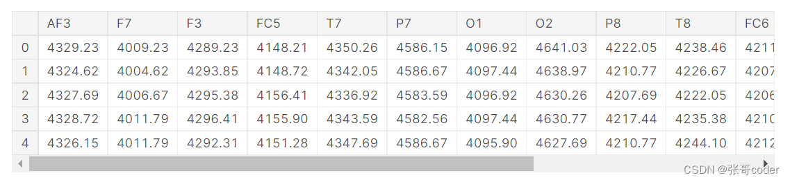
4 数据特征和标签的划分
# separate targets so you can preprocess the EEG data easily
Y = df['eyeDetection']
print( Y.shape )X = df.drop(columns='eyeDetection')
print( X.shape )
X.head()
(14980,)
(14980, 14)
5 识别脑电中的异常信号并使用差值的方法修正异常值
# Find outliers and put Nan instead
X = X.apply(stats.zscore, axis=0)
X = X.applymap(lambda x: np.nan if (abs(x) > 4) else x )# recalculate outliers with ignoring nans since the first calculation was biased with the huge outliers!
X = X.apply(stats.zscore, nan_policy='omit', axis=0)
X = X.applymap(lambda x: np.nan if (abs(x) > 4) else x )plot_data([X]) 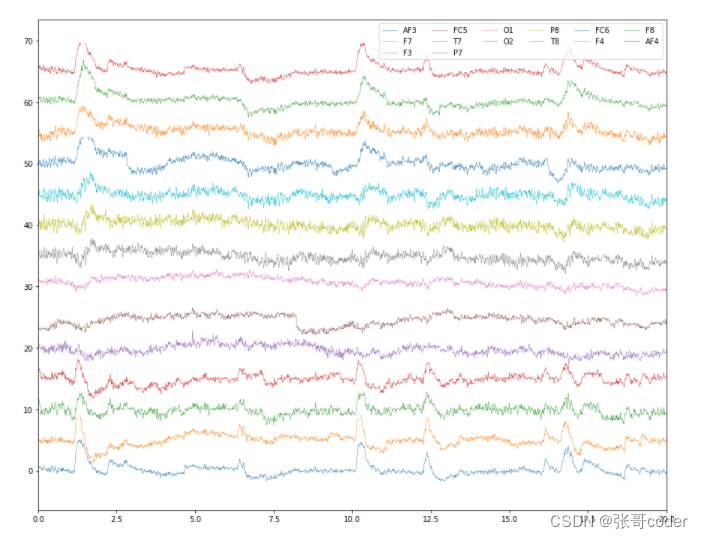
from scipy import signal, interpolatedef interp(x):t_temp = t[ x.index[ ~x.isnull() ] ]x = x[ x.index[ ~x.isnull() ] ]clf = interpolate.interp1d(t_temp, x, kind='cubic')return clf(t)# interpolate the nans using cubic spline method
X_interp = X.apply(interp, axis=0)plot_data([X_interp])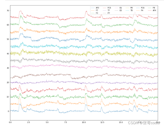
6 ICA, 数据独立成分分析
# ICA
from sklearn.decomposition import FastICA# apply ICA to drop non-electrophysiolgoical components (requires familiarity with EEG data)
ica = FastICA(max_iter=2000, random_state=0)
X_pcs = pd.DataFrame( ica.fit_transform(X_interp) )
X_pcs.columns = ['PC' + str(ind+1) for ind in range(X_pcs.shape[-1])]
X_pcs = X_pcs.drop(columns=['PC1', 'PC7'])
plot_data([X_pcs], xlim=[0, 120])# reconstruct clean EEG after dropping the bad components
ica.mixing_ = np.delete(ica.mixing_, [0, 6], axis = 1)
X_interp_clean = pd.DataFrame( ica.inverse_transform(X_pcs) )
X_interp_clean.columns = colsplot_data([X_interp, X_interp_clean], xlim=[0, 20])

7 从预处理数据中提取alpha脑电波信号
# now that data is clean, extract alpha waves magnitude from the clean signals# filter the data between 8-12 Hz (note that data has been rescaled to original scale after filtering for comparable visualization)
b, a = signal.butter(6, [8 / Fs * 2, 12 / Fs * 2], btype='bandpass')
X_interp_clean_alpha = X_interp_clean.apply(lambda x: signal.filtfilt(b, a, x) / max(abs(signal.filtfilt(b, a, x))) * max(abs(x)), axis=0)# extract envelope of the Alpha waves
X_interp_clean_alpha = X_interp_clean_alpha.apply(lambda x: np.abs(signal.hilbert(x)), axis=0)
X_interp_clean_alpha.columns = colsplot_data([X_interp_clean, X_interp_clean_alpha], xlim=[0, 10])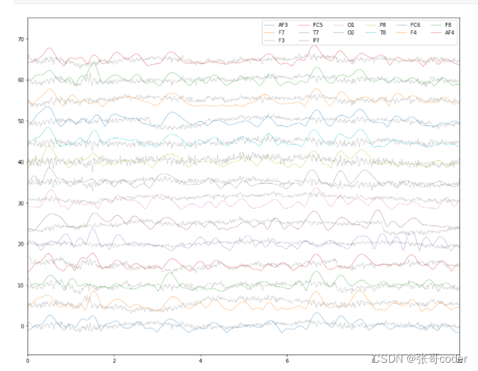
8 剔除高度相关的数据特征信号
# drop features with high correlations
X = X_interp_clean_alpha
Cols_corr = X.corr()# plot correlations of the cols
plt.figure( figsize=(10,10) )
sns.heatmap(Cols_corr, annot=True, annot_kws={'fontsize':12})# exclude columns with high correlation
cols_drop_ind = [0] * len(cols)
for i in range(len(cols)):for j in range(len(cols)):if (i<j) & abs( Cols_corr.iloc[i, j] >= 0.8):cols_drop_ind[j] = 1cols_drop = [cols[ind] for ind in range(len(cols_drop_ind)) if cols_drop_ind[ind]]
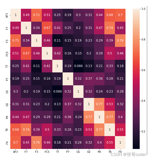
X.drop(columns=cols_drop, inplace=True)plt.figure( figsize=(10,10) )
sns.heatmap(X.corr(), annot=True, annot_kws={'fontsize':12})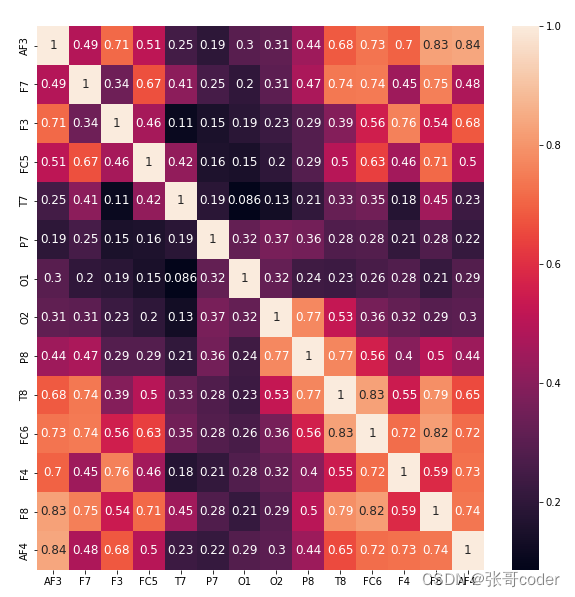
9 查看特征的线性分布特性
# just to check if the labels are linearly separable with less features! (Seems like we can't!)from sklearn.decomposition import PCA
from matplotlib import interactiveN = 2
pca = PCA(n_components=N)
X_pca = pd.DataFrame( pca.fit_transform(X), columns=['PC' + str(i+1) for i in range(N)])
print( 'Variance ratio explained by the components is :' + str(pca.explained_variance_ratio_))fig = plt.figure(figsize=(5,5))
ax = fig.add_subplot()
_ = ax.scatter(X_pca['PC1'], X_pca['PC2'], s = 1, c=Y, cmap='seismic', alpha=0.1)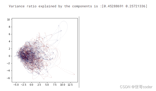
10 使用非线性核分类器实现数据的分类
# train an SVM to classify
from sklearn.svm import SVC
from sklearn.model_selection import train_test_split, GridSearchCV
from sklearn.preprocessing import StandardScaler# split train test data
X_train, X_test, y_train, y_test = train_test_split(X, Y, random_state=48, test_size=0.2, stratify=Y, shuffle=True)# normalize the features
scaler = StandardScaler()
X_train = scaler.fit_transform(X_train)
X_test = scaler.transform(X_test)
11 计算分类结果的指标
from sklearn.metrics import roc_auc_score# train with grid search
svc = SVC()
parameters = {'gamma': [0.1, 1, 10], 'C': [0.1, 1, 10]}
clf = GridSearchCV(svc, parameters)
clf.fit(X_train, y_train)# predict labels
y_pred = clf.predict(X_test)# extract accuracy (r2 score)
results = roc_auc_score(y_test, y_pred)# print score
print( 'Score is: ' + str( results ) )
print( 'Best params for the kernel SVM is: ' + str(clf.best_params_) )
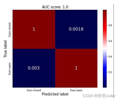
12 绘制分类结果混沌矩阵
from sklearn.metrics import confusion_matrix# confusion matrix estimation
conf = confusion_matrix(y_test, y_pred, normalize='true')plt.figure(figsize=(8,6))
sns.heatmap(conf, annot=True, cmap='seismic', annot_kws={'fontsize':18})
_ = plt.title( 'AUC score: ' + str(round(results, 2) ), fontsize=15)
_ = plt.xticks(ticks=[0.5, 1.5], labels=['Eyes-closed', 'Eyes-open'])
_ = plt.yticks(ticks=[0.5, 1.5], labels=['Eyes-closed', 'Eyes-open'])
_ = plt.ylabel('True label', fontsize=15)
_ = plt.xlabel('Predicted label', fontsize=15)