python零基础实现基于旋转特征的自监督学习(二)——在resnet18模型下应用自监督学习

系列文章目录
基于旋转特征的自监督学习(一)——算法思路解析以及数据集读取
基于旋转特征的自监督学习(二)——在resnet18模型下应用自监督学习
模型搭建与训练
- 系列文章目录
- 前言
- resNet18
-
- Residual
- resnet_block
- resNet18
- select_model
- 模型训练
-
- 损失函数与精度
- 批量训练
- 训练参数
- 效果对比
- 总结
前言
在本系列的上一篇文章中,我们介绍了如何对数据加载器进行修改来构建适合预基于特征旋转的自监督学习使用的数据集,在本篇文章中,我们将构建一个简易的深度学习模型——resnet18作为测试模型作为案例,在resnet18上我们进行训练,以及效果的对比。
代码地址:https://github.com/AiXing-w/little-test-for-FeatureLearningRotNet
resNet18
为了能够尽快看到结果,我们将搭建resNet18网络模型进行测试,这里我们将resnet18的搭建分为三个部分
residual、resnet_block、和resnet18。
其中resnet18是我们需要构建的模型,在之前的文章中我们曾经介绍过resnet模型的结构
可参考:常用结构化CNN模型构建
由于resnet18的模型结构是结构化的,为了方便表达,我们将模型分成多个块,即resnet_block;resnet_block也可以分成多个残差块,即residual。
Residual

Residual的实际就是两个卷积网络再加一个残差边,经过残差边的特征与经过卷积的特征相加再进行输出。
class Residual(nn.Module):def __init__(self, input_channels, num_channels, use_1x1conv=False, strides=1):super().__init__()self.conv1 = nn.Conv2d(input_channels, num_channels, kernel_size=3, padding=1, stride=strides)self.conv2 = nn.Conv2d(num_channels, num_channels, kernel_size=3, padding=1)if use_1x1conv:self.conv3 = nn.Conv2d(input_channels, num_channels, kernel_size=1, stride=strides)else:self.conv3 = Noneself.bn1 = nn.BatchNorm2d(num_channels)self.bn2 = nn.BatchNorm2d(num_channels)def forward(self, X):Y = F.relu(self.bn1(self.conv1(X)))Y = self.bn2(self.conv2(Y))if self.conv3:X = self.conv3(X)Y += Xreturn F.relu(Y)
resnet_block
使用resnet_block实现残差块(residual)的拼接,他需要传入三个参数:输入通道、输出通道、总共层数。一个可选参数first_block默认为False,用于判断是否为第一个resnet块。
def resnet_block(input_channels, num_channels, num_residuals, first_block=False):blk = []for i in range(num_residuals):if i == 0 and not first_block:blk.append(Residual(input_channels, num_channels, use_1x1conv=True, strides=2))else:blk.append(Residual(num_channels, num_channels))return blk
resNet18
使用resnet_block构建resnet18网络。
def resNet18(in_channels, num_classes):b1 = nn.Sequential(nn.Conv2d(in_channels, 64, kernel_size=7, stride=2, padding=3),nn.BatchNorm2d(64), nn.ReLU(),nn.MaxPool2d(kernel_size=3, stride=2, padding=1))b2 = nn.Sequential(*resnet_block(64, 64, 2, first_block=True))b3 = nn.Sequential(*resnet_block(64, 128, 2))b4 = nn.Sequential(*resnet_block(128, 256, 2))b5 = nn.Sequential(*resnet_block(256, 512, 2))net = nn.Sequential(b1, b2, b3, b4, b5,nn.AdaptiveAvgPool2d((1, 1)),nn.Flatten(),nn.Linear(512, num_classes))return net
select_model
为了后边可以拓展新的模型,所以我们构建一个select_model函数来用于选择模型
def select_model(model_name=str, kwargs=dict):# 选择模型if model_name == 'resNet18':net = resNet18(kwargs['in_channels'], kwargs['num_classes'])if os.path.exists("./model_weights/{}.pth".format(model_name)):net.load_state_dict(torch.load("./model_weights/{}.pth".format(model_name)))print("model wieghts loaded")return net
模型训练
损失函数与精度
Focal loss
如果仅使用交叉熵(cross entropy)的话有可能某些较为容易被学会的类别越学越好,然而其他类别越学越差。或者会受到数据不均衡的影响。所以我们将使用focal loss,可以抑制当时学习较好的样本,促进当时学习较差的样本。
import torch
from torch import nndef Focal_loss(pred, target,  alpha=0.5, gamma=2):logpt = -nn.CrossEntropyLoss(reduction='none')(pred, target)pt = torch.exp(logpt)if alpha is not None:logpt *= alphaloss = -((1 - pt)  gamma) * logptloss = loss.mean()return loss
accuracy
我们使用accuracy函数获取精度,他需要传入两个参数,y_hat和y。其中y_hat是预测结果,y是标签。
我们通过argmax获取y_hat中最大概率的预测,与y做比较。这个函数本质上就是用来评价有多少预测正确。
def accuracy(y_hat, y):# 预测精度if len(y_hat.shape) > 1 and y_hat.shape[1] > 1:y_hat = torch.argmax(y_hat, axis=1)cmp = y_hat.type(y.dtype) == yreturn float(cmp.type(y.dtype).sum()) / len(y)
批量训练
这个函数参数比较复杂
| 参数 | 含义 |
|---|---|
| net | 模型 |
| train_iter | 训练数据 |
| test_iter | 测试数据 |
| start | 起始轮次(开始训练的轮次) |
| num_epochs | 总轮次 |
| lr | 学习率 |
| device | 选择在cuda或cpu下训练 |
| threshold | 阈值(满足阈值设置时提前结束训练) |
| save_checkpoint | 选择是否按照检查点保存模型权值 |
| save_steps | 每隔几个轮次保存一次模型权值 |
| model_name | 保存权值时模型的名称 |
先使用Xavier初始化权值然后训练和测试模型即可,这里使用history来保存训练损失、训练精度、测试损失、测试精度
def train(net, train_iter, test_iter, start, num_epochs, lr, device, threshold, save_checkpoint=False, save_steps=50, model_name="rotation"):# 训练模型def init_weights(m):if isinstance(m, nn.Linear) or isinstance(m, nn.Conv2d):nn.init.xavier_uniform_(m.weight)net.apply(init_weights)print("device in : ", device)net = net.to(device)loss = nn.CrossEntropyLoss()history = {'train_loss': [], 'train_acc': [], 'test_loss': [], 'test_acc': []}optimizer = torch.optim.SGD(net.parameters(), lr=lr)for epoch in range(start, num_epochs):net.train()train_loss = 0.0train_acc = 0.0data_num = 0with tqdm(range(len(train_iter)), ncols=100, colour='red',desc="{} train epoch {}/{}".format(model_in_use, epoch + 1, num_epochs)) as pbar:for i, (X, y) in enumerate(train_iter):optimizer.zero_grad()X, y = X.to(device), y.to(device)y_hat = net(X)l = loss(y_hat, y)l.backward()optimizer.step()train_loss += l.detach()train_acc += accuracy(y_hat.detach(), y.detach())data_num += 1pbar.set_postfix({'loss': "{:.4f}".format(train_loss / data_num), 'acc': "{:.4f}".format(train_acc / data_num)})pbar.update(1)history['train_loss'].append(float(train_loss / data_num))history['train_acc'].append(float(train_acc / data_num))net.eval()test_loss = 0.0test_acc = 0.0data_num = 0with tqdm(range(len(test_iter)), ncols=100, colour='blue',desc="{} test epoch {}/{}".format(model_in_use, epoch + 1, num_epochs)) as pbar:for X, y in test_iter:X, y = X.to(device), y.to(device)y_hat = net(X)with torch.no_grad():l = loss(y_hat, y)test_loss += l.detach()test_acc += accuracy(y_hat.detach(), y.detach())data_num += 1pbar.set_postfix({'loss': "{:.4f}".format(test_loss / data_num), 'acc': "{:.4f}".format(test_acc / data_num)})pbar.update(1)history['test_loss'].append(float(test_loss / data_num))history['test_acc'].append(float(test_acc / data_num))if history['test_acc'][-1] > threshold:print("early stop")breakif save_checkpoint and (epoch+1) % save_steps == 0:torch.save(net.state_dict(), "./model_weights/{}-ep{}-{}-acc-{:.4f}-loss-{:.4f}.pth".format(model_name, epoch+1, model_in_use, history['test_acc'][-1], history['test_loss'][-1]))torch.save(net.state_dict(), "./model_weights/{}-{}.pth".format(model_in_use, model_name))return history
训练参数
基于旋转特征的自监督学习的参数
| 参数 | 含义 |
|---|---|
| batch_size | 批量大小 |
| in_channels | 输入通道数 |
| num_classes | 预测类别 |
| num_rotation_epochs | 自监督轮次数 |
| num_supervise_epochs | 迁移轮次数 |
| lr | 学习率 |
| threshold | 提前停止的阈值,即测试精度超过这个阈值就停止训练 |
| model_in_use | 使用的模型 |
| model_kargs | 模型参数,即输入通道数和总类别 |
| device | 测试cuda是否可用 |
| img_size | 改变图像大小 |
| is_freeze | 选择是否冻结自监督学习到的卷积层 |
这里可以看到,整个的训练过程需要加载两次数据并且训练两次,第一次是加载基于旋转特征的自监督学习的数据集,即判断是否经过旋转的数据集。另一次是加载cifar-10分类数据集(判断是否经过旋转的数据集也是cifar-10数据集,只不过我们在上一篇文章中在数据加载阶段对标签进行了修改)
if __name__ == '__main__':batch_size = 4086 # 批量大小in_channels = 3 # 输入通道数num_classes = 10 # 预测类别num_rotation_epochs = 100 # 自监督轮次num_supervise_epochs = 100 # 迁移lr = 2e-1threshold = 0.95 # 提前停止的阈值,即测试精度超过这个阈值就停止训练model_in_use = 'resNet18' model_kargs = {'in_channels': in_channels, "num_classes": 4} # 模型参数,即输入通道数和总类别device = 'cuda' if torch.cuda.is_available() else 'cpu' # 测试cuda并使用img_size = Noneis_freeze = Falsetrans = [transforms.ToTensor(), transforms.Normalize(mean=[x/255.0 for x in [125.3, 123.0, 113.9]],std=[x/255.0 for x in [63.0, 62.1, 66.7]])]trans = transforms.Compose(trans)train_iter, test_iter = LoadRotationDataset(batch_size=batch_size, trans=trans) # 加载数据集net = select_model(model_in_use, model_kargs)history = train(net, train_iter, test_iter, 0, num_rotation_epochs, lr, device, threshold, save_checkpoint=True) # 训练if is_freeze:for param in net.named_parameters():param[1].requires_grad = Falseif model_in_use == 'resNet18':net = net[:-3]net.add_module("new Adapt", nn.AdaptiveAvgPool2d((1, 1)))net.add_module("new Flatten", nn.Flatten())net.add_module("new linear", nn.Linear(512, num_classes))lr=2e-1train_iter, test_iter = LoadSuperviseDataset(batch_size=batch_size, trans=trans) # 加载数据集history_1 = train(net, train_iter, test_iter, num_rotation_epochs, num_rotation_epochs+num_supervise_epochs, lr, device, threshold, save_checkpoint=True) # 训练for key in list(history.keys()):history[key] = history[key] + history_1[key]plot_history(model_in_use + "_rotation", history)
监督学习的参数
如果不使用基于特征旋转的自监督学习,那么我们只需要去掉下面几行代码即可,同时要注意将history修改到与plot_history中使用的名称保持一致。
train_iter, test_iter = LoadRotationDataset(batch_size=batch_size, trans=trans)  # 加载数据集
net = select_model(model_in_use, model_kargs)
history = train(net, train_iter, test_iter, 0, num_rotation_epochs, lr, device, threshold,save_checkpoint=True)  # 训练
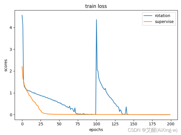
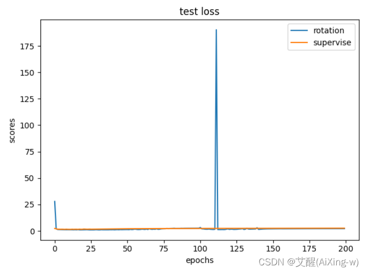
效果对比
完成训练后,在项目所在的文件夹中会生成txt文件来存储训练过程中产生的训练精度、训练损失、测试精度、测试损失。我们写一个函数来对比这些数据
import matplotlib.pyplot as pltdef compare(rotationName, superviseName, titleName):rotation_acc = []with open(rotationName) as f:for acc in f.readlines():rotation_acc.append(float(acc.strip()))supervise_acc = []with open(superviseName) as f:for acc in f.readlines():supervise_acc.append(float(acc.strip()))plt.plot(range(len(rotation_acc)), rotation_acc, label='rotation')plt.plot(range(len(supervise_acc)), supervise_acc, label='supervise')plt.xlabel('epochs')plt.ylabel('scores')plt.title(titleName)plt.legend()plt.show()if __name__ == "__main__":compare("resNet18_rotation_test_acc.txt", "resNet18_supervise_test_acc.txt", "test acc")compare("resNet18_rotation_test_loss.txt", "resNet18_supervise_test_loss.txt", "test loss")
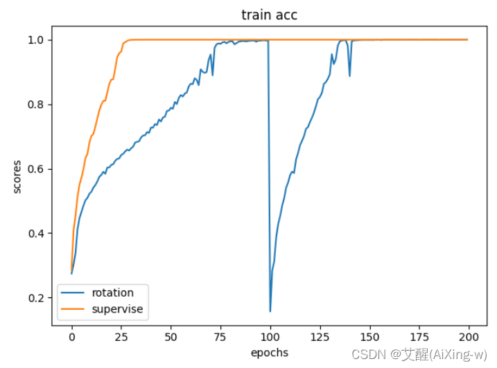
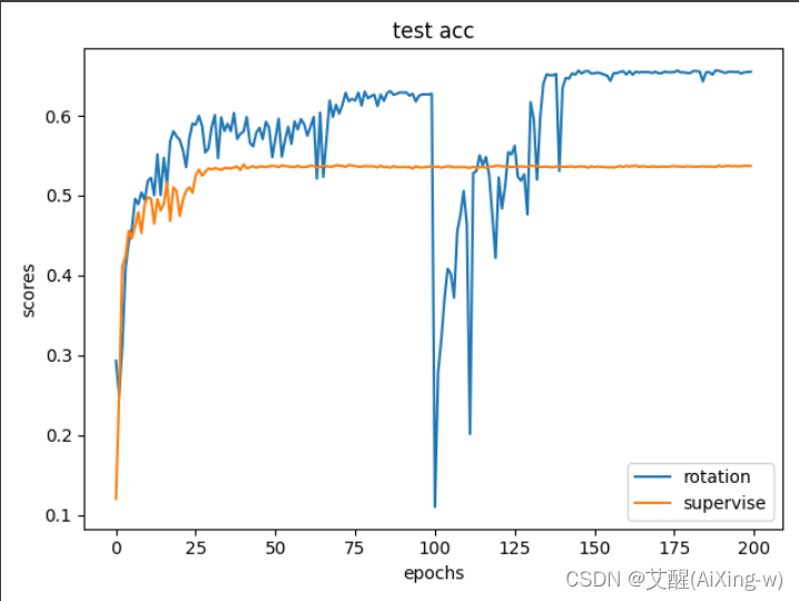
可以看到虽然在其他指标中两者差距并不明显,但是在测试精度(test acc)中使用了基于旋转特征的自监督学习的精度上升十分明显。
总结
基于旋转特征的自监督学习实质上就是将原始图像进行旋转,旋转过后将他的标签设置成旋转的角度。然后传入模型进行训练,训练好的权值作为分类模型的预训练模型进行模型迁移。